
Research研究

LLaVA-OneVision-1.5

Fully Open Framework for Democratized Multimodal Training完全开放的普惠多模态训练框架

LLaVA-OneVision-1.5 is a family of open vision–language models (3B, 4B and 8B) whose whole training recipe is public: an 85M-sample concept-balanced mid-training set, a 22M-sample instruction set, and the code, configurations and logs used to train them. The full pipeline fits a $16,000 compute budget, and the 8B model beats Qwen2.5-VL-7B on 18 of 27 benchmarks.

LLaVA-OneVision-1.5 是一组开源视觉语言模型(3B、4B、8B),完整训练配方全部公开:8500 万样本的概念均衡中期训练集、2200 万样本的指令集,以及训练所用的代码、配置和日志。整套流程的算力预算不超过 1.6 万美元,8B 模型在 27 个基准中的 18 个上超过 Qwen2.5-VL-7B。

The LLaVA JourneyLLaVA 之旅

LLaVA connected an open vision encoder to a large language model through a cheap alignment stage, and each successor widened what that recipe covers: cleaner data and higher resolution in LLaVA-1.5[24], OCR and math in LLaVA-NeXT[25], video in LLaVA-NeXT-Video[26], multi-image reasoning in LLaVA-NeXT-Interleave[27], and one interface for images, documents, charts and video in LLaVA-OneVision[28].

LLaVA 用一个低成本的对齐阶段把开源视觉编码器接到大语言模型上,之后每一代都扩展了这套配方的覆盖面:LLaVA-1.5[24] 带来更干净的数据和更高的分辨率,LLaVA-NeXT[25] 扩展到 OCR 与数学,LLaVA-NeXT-Video[26] 加入视频,LLaVA-NeXT-Interleave[27] 支持多图推理,LLaVA-OneVision[28] 则用一个接口统一了图像、文档、图表和视频。

Strong models such as Qwen2.5-VL[46] and InternVL3.5[48] publish weights but only part of their data recipes, mixing ratios and schedules, so they cannot be reproduced end to end. The remaining gap is in recipes and engineering, not in architecture. LLaVA-OneVision-1.5 releases all three missing pieces: the data, an efficient training framework (offline packing and hybrid parallelism), and the models together with the commands that reproduce their evaluation.

Qwen2.5-VL[46]、InternVL3.5[48] 等强模型公开了权重,但数据配方、混合比例和训练调度只部分公开,无法端到端复现。如今的差距在配方与工程,而不在架构。LLaVA-OneVision-1.5 把缺失的三部分全部公开:数据、高效训练框架(离线打包与混合并行),以及模型和复现其评测结果的命令。

Architecture模型架构

The model keeps LLaVA's ViT–MLP–LLM design. The vision encoder is RICE-ViT[47]; a projector merges each 2×2 group of neighbouring patches and maps it into the embedding space of a Qwen3 language model. RICE-ViT uses 2D RoPE[49], so every image is encoded at its native resolution rather than resized or tiled. Images of different sizes are packed into one sequence and attend only to their own tokens (Figure 1).

模型沿用 LLaVA 的 ViT–MLP–LLM 结构。视觉编码器为 RICE-ViT[47];投影层把每 2×2 个相邻 patch 合并,并映射到 Qwen3 语言模型的嵌入空间。RICE-ViT 采用二维 RoPE[49],每张图都以原生分辨率编码,不做缩放或切块。不同尺寸的图像被打包进同一条序列,且只在各自的 token 内做注意力(图 1)。

Figure 1. Overall architecture (after Figure 2 of the technical report). A photo, a chart, an equation and a document page each keep their native resolution, so they become different numbers of vision tokens. They are packed into one sequence without resizing or padding, self-attention in RICE-ViT stays within each image, and the MLP projector merges every 2×2 patch group into one token for the language model.图 1. 整体架构(参照技术报告图 2)。照片、图表、公式和文档页都保持原生分辨率,因此产生的视觉 token 数各不相同。它们不经缩放、不加填充地打包进同一条序列;RICE-ViT 中的自注意力只在每张图内部进行;MLP 投影器把每 2×2 个 patch 合并为一个 token,再送入语言模型。

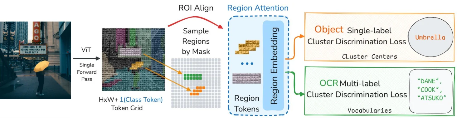
Contrastive encoders such as CLIP[37] and SigLIP[41] align one global vector per image with its caption, which says little about individual objects or lines of text. RICE-ViT is instead trained by region cluster discrimination on 450M images and 2.4B candidate regions: object regions and OCR regions learn to predict their clusters, so one objective covers semantics, text recognition and localisation. With the encoder swapped into the same pipeline, it has the best OCR and document scores of the encoders compared.

CLIP[37]、SigLIP[41] 等对比学习编码器只把整张图的一个全局向量与文本对齐,难以刻画单个物体或一行文字。RICE-ViT 改用区域聚类判别训练,数据为 4.5 亿张图像和 24 亿个候选区域:物体区域与 OCR 区域学习预测各自所属的聚类,一个目标同时覆盖语义、文字识别与定位。在同一流程中替换编码器后,它在 OCR 与文档基准上取得了所比较编码器中的最好成绩。

How RICE-ViT is trained, and the encoder comparison (Figure 2, Table 1)RICE-ViT 的训练方式与编码器对比(图 2、表 1)
RICE-ViT training: a ViT token grid, region sampling with ROI Align, region attention, and object and OCR cluster-discrimination losses
Figure 2. How RICE-ViT is trained (from the RICE paper[47]). One forward pass of the ViT yields a token grid; regions are sampled by mask with ROI Align, region attention turns each into a fixed-length embedding, and object regions and OCR regions are supervised by single-label and multi-label cluster discrimination.图 2. RICE-ViT 的训练方式(取自 RICE 论文[47])。ViT 一次前向得到 token 网格;按掩码用 ROI Align 采样区域,区域注意力把每个区域变成定长嵌入,物体区域和 OCR 区域分别由单标签与多标签聚类判别监督。

SigLIP2[45] reaches dense features by combining several specialised losses (SILC[42], TIPS[43], LocCa[44]); RICE-ViT gets semantics, text recognition and localisation from the single cluster-discrimination objective. Table 1 swaps encoders inside the same LLaVA-NeXT pipeline. At every resolution RICE-ViT, a ViT-L, has the best OCR and document average, ahead of the larger SigLIP and SigLIP2 SO400M towers; the RICE-ViT taken from LLaVA-OV-1.5-3B also beats the Qwen-ViT of Qwen2.5-VL-7B on both averages (64.8 vs 62.9 and 73.4 vs 72.5).

SigLIP2[45] 依靠多个专用损失(SILC[42]、TIPS[43]、LocCa[44])获得稠密特征;RICE-ViT 只用一个聚类判别目标就同时获得语义、文字识别和定位能力。表 1 在同一 LLaVA-NeXT 流程中替换编码器:在每个分辨率下,ViT-L 规模的 RICE-ViT 的 OCR 与文档平均分都最高,超过更大的 SigLIP、SigLIP2 SO400M;取自 LLaVA-OV-1.5-3B 的 RICE-ViT 在两项平均分上也都超过 Qwen2.5-VL-7B 的 Qwen-ViT(64.8 对 62.9,73.4 对 72.5)。

Table 1RICE-ViT against other vision encoders in the LLaVA-NeXT framework: Qwen2.5-7B as the language model, LLaVA-NeXT training data and the same training pipeline for every row. RICE-ViT rows are shaded.表 1在 LLaVA-NeXT 框架中对比 RICE-ViT 与其他视觉编码器:每一行都使用 Qwen2.5-7B 语言模型、LLaVA-NeXT 训练数据和相同的训练流程。RICE-ViT 所在行加底色。
Model Configuration OCR & Document Understanding General Vision Understanding
Method Vision Tower
InfoVQA
DocVQA
ChartQA
TextVQA
OCRBench
OCRBenchV2
LiveXivVQA
OCR Avg
AI2D
MMBEN
MMECog
MMEPer
POPE
RealworldQA
MMStar
Other Avg
CLIP[37] ViT-L-14-336px 38.9 75.2 66.5 62.5 52.5 23.0 47.4 52.3 73.2 74.6 48.0 75.6 88.8 63.7 49.0 67.6
MLCD[38] ViT-L-14-336px 43.5 76.5 67.8 61.7 53.1 24.0 48.4 53.6 77.0 76.4 54.1 79.9 88.7 61.1 51.0 69.7
AIMv2[39] ViT-L-14-336px 35.4 77.2 72.7 65.9 57.2 23.9 47.3 54.2 75.4 78.6 48.3 75.0 88.4 62.2 50.2 68.3
RICE-ViT ViT-L-14-336px 45.2 79.2 72.3 65.9 57.5 24.1 48.9 56.2 77.9 76.6 54.6 80.7 88.5 63.1 51.8 70.5
DFN5B[40] ViT-H-14-378px 38.6 70.9 64.4 59.4 47.3 21.9 46.2 49.8 73.5 73.4 45.8 76.9 88.6 59.9 49.1 66.7
SigLIP[41] ViT-SO400M-14-384px 41.4 76.7 69.3 64.7 55.4 24.0 48.4 54.3 76.2 77.0 46.1 79.9 88.8 63.7 47.3 68.4
SigLIPv2[45] ViT-SO400M-14-384px 43.7 79.1 70.2 66.2 58.7 25.4 48.6 56.0 77.0 77.1 46.6 80.4 89.3 63.4 52.8 69.5
RICE-ViT ViT-L-14-378px 48.1 82.6 75.1 66.2 58.8 25.8 49.5 58.0 76.5 77.6 54.1 79.0 89.1 62.9 51.2 70.1
SigLIPv2[45] ViT-SO400M-16-560px 50.2 86.2 77.4 70.2 62.7 26.5 52.9 60.9 77.0 76.5 53.5 79.9 89.3 68.2 53.1 71.1
RICE-ViT ViT-L-14-560px 53.2 87.4 78.1 69.0 60.7 26.1 53.0 61.1 76.9 78.6 56.3 79.3 88.9 65.1 50.5 70.8
Qwen-ViT from Qwen2.5-VL 7B[46] ViT-H-14-560px 55.9 85.8 78.8 73.7 66.2 26.8 53.4 62.9 78.8 78.4 62.0 80.8 88.6 64.2 55.0 72.5
RICE-ViT from OV-1.5 3B ViT-L-14-560px 53.7 87.1 81.9 73.8 73.3 30.4 53.6 64.8 80.3 79.6 58.6 82.2 89.0 67.3 56.6 73.4

Data数据

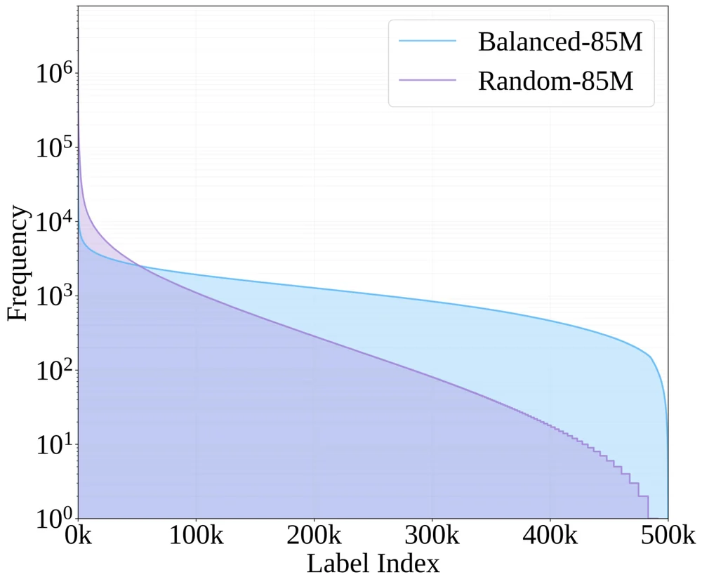
Mid-training uses 85M image–caption pairs, 65M in English and 20M in Chinese, from eight sources: COYO-700M[29], Obelics[30], DataComp-1B[31], LAION-CN[32], ImageNet-21K[33], SAM-1B[34], MINT[35] and Zero250M[36]. Raw web captions over-represent common concepts and leave rare ones sparse, so the set is concept-balanced: a MetaCLIP encoder embeds every image and a 500K-concept vocabulary in one space, each image is tagged with its top-K nearest concepts, and images are resampled with weights inverse to concept frequency. A captioner then writes new bilingual captions for the selected images. Figure 3a shows the long tail flattening.

中期训练使用 8500 万图文对(英文 6500 万、中文 2000 万),来自八个数据源:COYO-700M[29]、Obelics[30]、DataComp-1B[31]、LAION-CN[32]、ImageNet-21K[33]、SAM-1B[34]、MINT[35] 和 Zero250M[36]。原始网络描述偏向常见概念、稀有概念样本稀少,因此我们做概念均衡:用 MetaCLIP 编码器把所有图像和 50 万规模的概念词表嵌入同一空间,为每张图标注 Top-K 最近的概念,再按概念频率的倒数加权重采样。随后由描述模型为选中的图像重新生成中英双语描述。图 3a 显示长尾分布被拉平。

The 22M instruction set mixes general VQA, OCR, charts and tables, captions, science, code and math, grounding and counting, domain-specific tasks and text-only data (Figure 3c). Samples are aggregated from many sources, rewritten into consistent formats and templates, converted into both languages and safety-filtered; adding FineVision on top improves results further.

2200 万指令集涵盖通用 VQA、OCR、图表与表格、图像描述、科学、代码与数学、定位与计数、领域任务以及纯文本数据(图 3c)。样本从多个来源汇集,统一改写为一致的格式与模板,转换为中英两种语言,并做安全过滤;在此基础上加入 FineVision 还能进一步提升效果。

(a) Concept coverage(a) 概念覆盖
Concept frequency over the 500K vocabulary before and after balancing: the balanced curve is flatter
(b) Mid-training sources, 85M(b) 中期训练数据来源(85M)
MINT 5.0%
ImageNet-21K 1.9%
SA-1B 1.4%
(c) Instruction categories, 22M(c) 指令数据类别(22M)
Caption图像描述 4.8%
Science科学 4.1%
Code & math代码与数学 3.3%
Grounding定位与计数 0.6%
Figure 3. (a) Vocabulary coverage of the mid-training set before and after concept balancing. (b) Sources of the 85M mid-training set. (c) Categories of the 22M instruction set.图 3. (a) 概念均衡前后中期训练集的词表覆盖。(b) 8500 万中期训练集的数据来源。(c) 2200 万指令集的类别分布。
Data ablations: concept balancing and mid-training scale (Figures 4, 5)数据消融:概念均衡与中期训练规模(图 4、图 5)

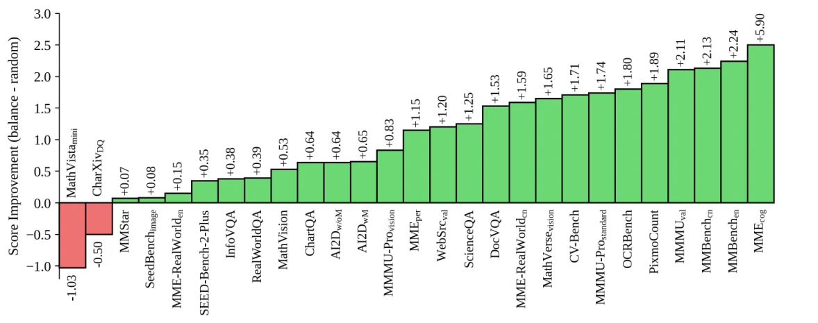
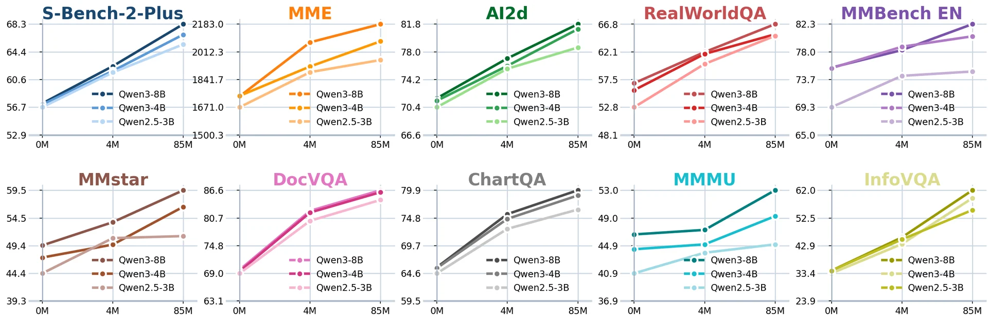
Both ablations pretrain on LLaVA-558K and fine-tune on LLaVA-NeXT-780K, changing only the mid-training data. With 2M mid-training samples, concept-balanced sampling beats random sampling on 25 of 27 benchmarks (Figure 4). Growing mid-training from none to 4M to 85M samples raises the scores of all three language models (Figure 5).

两组消融都在 LLaVA-558K 上预训练、在 LLaVA-NeXT-780K 上微调,只改变中期训练数据。使用 200 万中期训练样本时,概念均衡采样在 27 个基准中的 25 个上优于随机采样(图 4)。把中期训练从没有扩大到 400 万、再到 8500 万样本,三个语言模型的分数都随之上升(图 5)。

Score change from balanced over random sampling on 27 benchmarks: two drops, 25 gains
Figure 4. Score improvement of concept-balanced over random sampling (balanced − random) with 2M mid-training samples. Only MathVistamini (−1.03) and CharXivDQ (−0.50) drop; MMEcog gains most (+5.90).图 4. 概念均衡采样相对随机采样的分数提升(均衡 − 随机),中期训练样本为 200 万。只有 MathVistamini(−1.03)和 CharXivDQ(−0.50)下降;MMEcog 提升最多(+5.90)。
Scores on SEED-Bench-2-Plus, MME, AI2D, RealWorldQA, MMBench, MMStar, DocVQA, ChartQA, MMMU and InfoVQA rise from 0M to 4M to 85M mid-training samples for Qwen3-8B, Qwen3-4B and Qwen2.5-3B
Figure 5. Benchmark scores after mid-training on 0, 4M and 85M samples, for three language models. 0M means no mid-training stage.图 5. 三个语言模型在中期训练样本为 0、400 万、8500 万时的基准分数。0M 表示没有中期训练阶段。

Training训练

Training has three stages. Stage 1 trains only the projector, aligning visual features with the language model’s word embeddings. Stages 1.5 and 2 train all parameters: first on the 85M concept-balanced captions to add visual knowledge, then on the 22M instructions plus FineVision to teach tasks and answer formats.

训练分三个阶段。阶段 1 只训练投影层,把视觉特征与语言模型的词嵌入对齐。阶段 1.5 和阶段 2 训练全部参数:先在 8500 万概念均衡的图文描述上注入视觉知识,再在 2200 万指令数据与 FineVision 上学习任务和回答格式。

Stage 1

Language–image alignment语言-图像对齐

Projector only · LLaVA-1.5 558K仅训练投影层 · LLaVA-1.5 558K
→
Stage 1.5

Mid-training中期训练

Full model · concept-balanced 85M全参数 · 概念均衡 85M
→
Stage 2

Instruction tuning指令微调

Full model · 22M + FineVision全参数 · 22M + FineVision

Offline packing离线打包

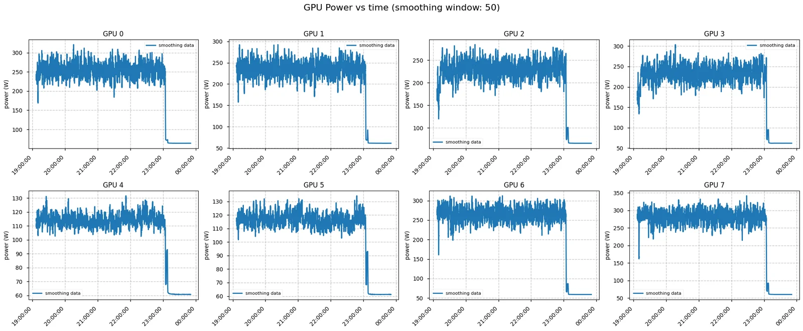
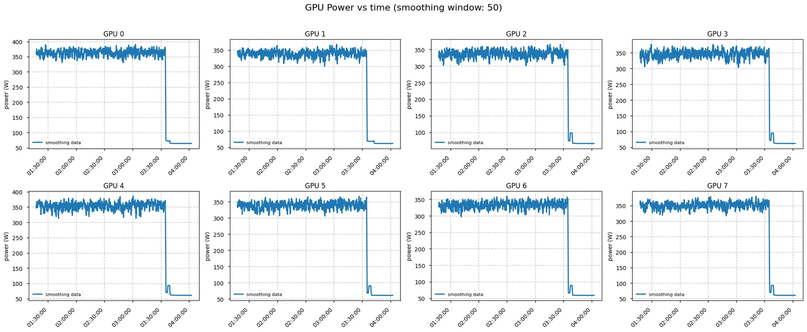
Multimodal samples vary widely in length. Padding them into batches wastes compute on padding tokens and makes fast GPUs wait for slow ones. LLaVA-OneVision-1.5 packs samples offline instead: before training, samples are bucketed by token length and concatenated into sequences that fill the context, and the result is written once and reused. On the 85M set this reduces padding by up to 11×. Figure 6 shows the effect on GPU power: without packing, power swings between roughly 100 and 300 W and two GPUs stay near 115 W, waiting; with packing all eight hold about 350 W.

多模态样本的长度差异很大。把它们填充后组成 batch,会把算力浪费在填充 token 上,也会让快的 GPU 等待慢的 GPU。LLaVA-OneVision-1.5 改为离线打包:训练前按 token 长度分桶,把样本拼接成填满上下文的序列,结果只写一次、反复使用。在 8500 万数据上,填充最多减少约 11 倍。图 6 显示了它对 GPU 功耗的影响:不打包时功耗在约 100 到 300 W 之间剧烈波动,有两块 GPU 停在约 115 W 等待;打包后八块 GPU 都稳定在约 350 W。

(a) Packing(a) 打包
Sample packing: several short samples are concatenated into one sequence of the target length instead of being padded one by one
(b) Without packing(b) 不打包
Power of eight GPUs during training on non-packed samples: large swings between about 100 and 300 W, and two GPUs near 115 W
(c) With offline packing(c) 离线打包
Power of eight GPUs during training on packed samples: all eight steady near 350 W
Figure 6. Offline packing. (a) Several short samples are concatenated into one sequence of the target length instead of each being padded. (b, c) Power of eight GPUs over a training run on non-packed and on packed samples (smoothing window 50). From the offline-packing example in the LLaVA-OneVision repository.图 6. 离线打包。(a) 多个短样本拼接成一条目标长度的序列,而不是各自填充。(b, c) 在未打包与打包样本上训练时八块 GPU 的功耗(平滑窗口 50)。取自 LLaVA-OneVision 仓库中的离线打包示例。
How the offline packer works离线打包器如何工作

The packer runs once over the whole corpus before training, in four steps:

打包器在训练前对整个语料运行一次,分四步:

  1. Split the source JSON into one file per sample.把源 JSON 拆成每个样本一个文件。
  2. Compute each sample’s token length with the model’s processor, so image tokens are counted exactly.用模型的 processor 计算每个样本的 token 长度,图像 token 也精确计入。
  3. Group samples into hash buckets by length and bin-pack them into sequences that fill the target context; long samples seed a bin and shorter ones fill the remainder, with multi-threaded scheduling over the global statistics.按长度把样本放入哈希桶,再装箱成填满目标上下文的序列;长样本作为种子占据一个箱,短样本填补剩余空间,基于全局统计多线程调度。
  4. Write the packed sequences and their sample boundaries to WebDataset shards, which the trainer reads directly.把打包后的序列及其样本边界写入 WebDataset 分片,训练时直接读取。

Online packing, as in LLaMA-Factory or Megatron, only sees a small rolling buffer inside the dataloader, so it finds fewer good fits and pays the search cost at every step; a larger buffer costs host memory and latency. Packing offline sees the whole shard, is deterministic and reproducible, and adds nothing to training time. Inside a packed sequence, samples are kept apart with FlashAttention’s variable-length kernels.

LLaMA-Factory、Megatron 中的在线打包只能看到 dataloader 里很小的滚动缓冲区,找到的互补样本更少,并且每一步都要付出搜索开销;扩大缓冲区又会增加主机内存和延迟。离线打包看到的是整个分片,结果确定、可复现,也不增加训练时间。在一条打包序列内部,各样本通过 FlashAttention 的变长 kernel 保持相互隔离。

Hybrid parallelism混合并行

The 8B model is trained in AIAK-Training-LLM, a Megatron-LM derivative, with tensor, pipeline and sequence parallelism, a distributed optimizer and uniform recomputation, at native resolution with an 8K context. On 128 A800 GPUs, mid-training on the 85M samples takes 3.7 days, and the whole pipeline stays within a $16,000 compute budget.

8B 模型在基于 Megatron-LM 的 AIAK-Training-LLM 中训练,采用张量并行、流水线并行、序列并行、分布式优化器和均匀重计算,以原生分辨率和 8K 上下文训练。在 128 块 A800 GPU 上,8500 万样本的中期训练耗时 3.7 天,整套流程的算力预算不超过 1.6 万美元。

Training time and loss curve (Figure 7)训练时长与损失曲线(图 7)
Training loss over time for Mid-Training and SFT phases with a logarithmic y-axis Mid-Training (89h) 中期训练 (89h) SFT (79h) SFT (79h)
Mid-training中期训练89.39h
SFT79.05h
Total总时长168.44h
Hardware硬件128 GPUs
Figure 7. Training loss of the 8B model over wall-clock time on 128 GPUs, log scale: mid-training (89 h), then SFT (79 h). Faint lines are raw logged loss, solid lines are smoothed.图 7. 8B 模型在 128 块 GPU 上的训练损失随时间变化(对数坐标):先中期训练(89 小时),再 SFT(79 小时)。浅色线为原始记录的损失,实线为平滑后的结果。

Results结果

Table 2 averages the 27 benchmarks of the full comparison (Table 3) by task group. LLaVA-OV-1.5-8B beats Qwen2.5-VL-7B on 18 of the 27 and leads three of the four groups. The margins are largest on general VQA (MMStar 67.7 vs 62.5) and chart understanding (CharXivDQ 74.1 vs 69.8); Qwen2.5-VL-7B stays ahead on InfoVQA, OCRBench, PixmoCount and VL-RewardBench. The smaller models gain more: the 4B model beats Qwen2.5-VL-3B on 26 of 27 benchmarks.

表 2 按任务类别对完整对比(表 3)中的 27 个基准求平均。LLaVA-OV-1.5-8B 在 27 个基准中的 18 个上超过 Qwen2.5-VL-7B,四个类别中领先三个。差距最大的是通用 VQA(MMStar 67.7 对 62.5)和图表理解(CharXivDQ 74.1 对 69.8);Qwen2.5-VL-7B 在 InfoVQA、OCRBench、PixmoCount 和 VL-RewardBench 上仍然领先。小模型的优势更明显:4B 模型在 27 个基准中的 26 个上超过 Qwen2.5-VL-3B。

Table 2Average score per task group (number of benchmarks in brackets). Blue marks the best average in a row.表 2各任务类别的平均分(括号内为基准数量)。蓝色表示该行最佳平均分。
Task group任务类别 LLaVA-OV-1.5 8B Qwen2.5-VL 7B LLaVA-OV-1.5 4B LLaVA-OV-1.5 3B Qwen2.5-VL 3B
General VQA (10)通用 VQA(10) 74.2 72.2 72.1 66.5 66.4
Reasoning (6)推理(6) 41.1 40.8 38.4 33.7 33.1
OCR & chart (7)OCR 与图表(7) 85.0 84.4 82.6 81.0 79.8
Others (4)其他(4) 68.8 69.1 63.8 54.1 58.8
Table 3Performance comparison across vision-language models on 27 benchmarks grouped by task type. All scores are accuracy (%) unless stated otherwise. Blue marks the best score in a row, including ties.表 3不同视觉语言模型在按任务类型分组的 27 个基准上的性能对比。除特别说明外均为准确率(%)。蓝色表示该行最佳(含并列)。
Benchmark LLaVA-OV-1.5 8B Qwen2.5-VL 7B LLaVA-OV-1.5 4B LLaVA-OV-1.5 3B Qwen2.5-VL 3B
MMStar[14] 67.7 62.5 64.9 59.1 55.9
MMBenchen[10] 84.1 83.4 84.2 81.0 78.0
MMBenchcn[10] 81.0 81.6 76.9 73.0 74.6
MME-RealWorlden[11] 62.3 57.3 49.6 57.9 51.6
MME-RealWorldcn[11] 56.1 51.5 61.6 23.4 45.4
SeedBenchimage[20] 77.3 77.5 76.6 71.3 74.8
CV-Bench[5] 80.8 80.0 77.2 73.8 71.5
ScienceQA[18] 95.0 88.8 93.6 91.2 83.3
SEED-Bench-2-Plus[19] 69.2 70.9 68.9 67.6 68.6
RealWorldQA[17] 68.1 68.5 67.8 66.8 60.0
Avg 74.2 72.2 72.1 66.5 66.4
MathVistamini[9] 69.6 68.6 67.9 64.7 60.2
WeMath[23] 33.6 33.3 24.9 22.6 18.4
MathVision[8] 25.6 22.4 24.2 19.9 21.3
MMMUval[12] 55.4 51.3 52.7 45.5 46.4
MMMU-Prostandard[13] 37.4 36.3 35.3 29.5 31.1
MMMU-Provision[13] 25.2 32.8 25.4 20.3 21.3
Avg 41.1 40.8 38.4 33.7 33.1
ChartQA[2] 86.5 84.1 87.1 84.4 83.4
CharXivDQ[3] 74.1 69.8 63.8 61.8 58.2
DocVQA[6] 95.0 94.9 94.4 93.4 92.7
OCRBench[15] 82.9 84.2 80.0 80.5 79.2
AI2DwM[1] 84.2 82.6 83.6 82.3 78.6
AI2Dw/oM[1] 94.1 93.4 93.3 91.9 90.7
InfoVQA[7] 78.4 81.7 76.1 71.2 75.6
Avg 85.0 84.4 82.6 81.0 79.8
PixmoCount[16] 62.2 63.3 52.2 57.0 50.9
CountBench[4] 88.2 86.4 79.8 49.5 72.5
VL-RewardBench[22] 46.7 49.7 48.2 42.5 42.1
V*[21] 78.0 77.0 74.9 67.5 69.6
Avg 68.8 69.1 63.8 54.1 58.8

Open-Source Resources开源资源

Weights, data and code are all public: the 8B model runs with Hugging Face Transformers, and a single lmms-eval command runs its evaluation.

权重、数据和代码全部公开:8B 模型可直接用 Hugging Face Transformers 运行,一条 lmms-eval 命令即可运行它的评测。

Quick start with Hugging Face (Python)用 Hugging Face 快速上手(Python)
Quick Start with HuggingFaceHuggingFace 快速开始
python
from transformers import AutoTokenizer, AutoProcessor, AutoModelForCausalLM
from qwen_vl_utils import process_vision_info

model_path = "lmms-lab/LLaVA-One-Vision-1.5-8B-Instruct"

# default: Load the model on the available device(s)

model = AutoModelForCausalLM.from_pretrained(
    model_path, torch_dtype="auto", device_map="auto", trust_remote_code=True
)

# default processor

processor = AutoProcessor.from_pretrained(model_path, trust_remote_code=True)

messages = [
    {
        "role": "user",
        "content": [
            {
                "type": "image",
                "image": "https://qianwen-res.oss-cn-beijing.aliyuncs.com/Qwen-VL/assets/demo.jpeg",
            },
            {"type": "text", "text": "Describe this image."},
        ],
    }
]

# Preparation for inference

text = processor.apply_chat_template(
    messages, tokenize=False, add_generation_prompt=True
)
image_inputs, video_inputs = process_vision_info(messages)
inputs = processor(
    text=[text],
    images=image_inputs,
    videos=video_inputs,
    padding=True,
    return_tensors="pt",
)
inputs = inputs.to("cuda")

# Inference: Generation of the output

generated_ids = model.generate(inputs, max_new_tokens=1024)
generated_ids_trimmed = [
    out_ids[len(in_ids) :] for in_ids, out_ids in zip(inputs.input_ids, generated_ids)
]
output_text = processor.batch_decode(
    generated_ids_trimmed, skip_special_tokens=True, clean_up_tokenization_spaces=False
)
print(output_text)
Evaluation command (lmms-eval)评测命令(lmms-eval)
Model Evaluation模型评估
bash
# pip install git+https://github.com/EvolvingLMMs-Lab/lmms-eval.git
accelerate launch --num_processes=8 --main_process_port 12399 -m lmms_eval \
 --model=llava_onevision1_5 \
 --model_args=pretrained=lmms-lab/LLaVA-OneVision-1.5-8B-Instruct,attn_implementation=flash_attention_2,max_pixels=3240000 \
 --tasks=mmmu_val,mmmu_pro_standard,mmbench_en_test,mmerealworld,mmerealworld_cn,ai2d,ai2d_no_mask,vstar_bench,chartqa,charxiv,docvqa_test,mathvista_testmini,mmstar,scienceqa \
 --batch_size=1

Citation引用

citation.bib
bibtex
@inproceedings{LLaVA-OneVision-1.5,
  title={LLaVA-OneVision-1.5: Fully Open Framework for Democratized Multimodal Training},
  author={An, Xiang and Xie, Yin and Yang, Kaicheng and Zhang, Wenkang and Zhao, Xiuwei and Cheng, Zheng and Wang, Yirui and Xu, Songcen and Chen, Changrui and Wu, Chunsheng and Tan, Huajie and Li, Chunyuan and Yang, Jing and Yu, Jie and Wang, Xiyao and Qin, Bin and Wang, Yumeng and Yan, Zizhen and Feng, Ziyong and Liu, Ziwei and Li, Bo and Deng, Jiankang},
  booktitle={arXiv},
  year={2025}
}

@inproceedings{xie2025region,
  title={Region-based Cluster Discrimination for Visual Representation Learning},
  author={Xie, Yin and Yang, Kaicheng and An, Xiang and Wu, Kun and Zhao, Yongle and Deng, Weimo and Ran, Zimin and Wang, Yumeng and Feng, Ziyong and Miles, Roy and Elezi, Ismail and Deng, Jiankang},
  booktitle={ICCV},
  year={2025}
}

@article{lillava,
  title={LLaVA-OneVision: Easy Visual Task Transfer},
  author={Li, Bo and Zhang, Yuanhan and Guo, Dong and Zhang, Renrui and Li, Feng and Zhang, Hao and Zhang, Kaichen and Zhang, Peiyuan and Li, Yanwei and Liu, Ziwei and Li, Chunyuan},
  journal={Transactions on Machine Learning Research},
  year={2024}
}
Research研究

LLaVA-OneVision-1.5-RL

Eliciting chain-of-thought reasoning with a lightweight RL stage用轻量 RL 阶段激发链式思维推理

LLaVA-OneVision-1.5-RL adds a reinforcement-learning stage on top of LLaVA-OneVision-1.5-8B-Instruct. It trains on 67K examples the model can already solve but not reliably, scores answers with rule-based rewards, and runs in two stages: answer-only RL, then chain-of-thought RL. Thinking mode lifts the reasoning average from 45.8 to 51.8; fast mode keeps OCR and chart scores unchanged and improves counting and grounding.

LLaVA-OneVision-1.5-RL 在 LLaVA-OneVision-1.5-8B-Instruct 之上增加一个强化学习阶段。它在 6.7 万条“模型已经会做、但做不稳”的样本上训练,用基于规则的奖励给回答打分,并分两个阶段进行:先仅答案 RL,再链式思维 RL。Thinking 模式把推理类平均分从 45.8 提升到 51.8;fast 模式保持 OCR 与图表分数不变,并提升计数与定位能力。

RL Data Strategy强化学习数据策略

The RL data is not new annotation. It is drawn from public sets (ViRL39K[50], Ref-L4[51], VigoRL-SA and VigoRL-SAT[52], PixmoCount[16], WebCode2M[53], UniSVG[54], InfoVQA[7] and AI2D[1]) and filtered with the instruct model itself. Two filters decide what stays:

RL 数据不是新标注的,而是取自公开数据集(ViRL39K[50]、Ref-L4[51]、VigoRL-SA 与 VigoRL-SAT[52]、PixmoCount[16]、WebCode2M[53]、UniSVG[54]、InfoVQA[7] 和 AI2D[1]),再用指令模型本身筛选。两道筛选决定哪些样本留下:

  • Discrepancy-driven selection. A large gap between Pass@N and Pass@1 means correct answers already appear among the model’s samples but not reliably on the first try. RL can turn that latent ability into consistent behaviour, so these tasks are kept; tasks the model already solves (high Pass@1) or cannot solve (low Pass@N) are dropped.差异驱动筛选。Pass@N 与 Pass@1 之间差距大,说明正确答案已经出现在模型的采样中,只是第一次作答做不稳。RL 能把这种潜在能力变成稳定的行为,因此保留这类任务;模型已经会做(Pass@1 高)或做不出来(Pass@N 低)的任务被剔除。
  • Reward-based sampling. The base model answers each prompt several times and every answer is scored. Prompts whose average reward is near 1 (trivial) or near 0 (unsolvable) are removed, which leaves medium-difficulty prompts with a useful learning signal.基于奖励的采样。基础模型对每个题目作答多次并逐一打分。平均奖励接近 1(太简单)或接近 0(不可解)的题目被移除,留下能提供有效学习信号的中等难度题目。

67K examples remain, 58% of them STEM (Figure 8a). Each example also records whether it is posed answer-only or with chain-of-thought, and the two training stages draw on that: stage 1 uses 19.9K answer-only examples, three quarters of them grounding; stage 2 uses 49.2K chain-of-thought examples, 79% of them STEM.

最终留下 6.7 万条样本,其中 58% 为 STEM(图 8a)。每条样本还记录了它是仅答案形式还是链式思维形式,两个训练阶段据此取数:阶段一使用 1.99 万条仅答案样本,其中四分之三是定位任务;阶段二使用 4.92 万条链式思维样本,其中 79% 为 STEM。

(a) All RL data, 67.0K(a) 全部 RL 数据(67.0K)
(b) Stage 1, answer-only, 19.9K(b) 阶段一:仅答案(19.9K)
(c) Stage 2, chain-of-thought, 49.2K(c) 阶段二:链式思维(49.2K)
STEMSTEM
Grounding定位
Spatial空间
Coding代码
Counting计数
OCR & diagramOCR 与图表
Figure 8. Task categories in the RL training data. (a) The whole 67K pool. (b) Stage 1, answer-only. (c) Stage 2, chain-of-thought.图 8. RL 训练数据的任务类别分布。(a) 全部 6.7 万条数据。(b) 阶段一:仅答案。(c) 阶段二:链式思维。

Reward System Architecture奖励系统架构

Rewards come from rules, not from a learned preference model. Each answer type has its own checker in the reward/ module (Table 4): math answers are parsed and checked for symbolic equivalence, so ½, 0.5 and 2/4 all match; boxes are scored by IoU; code by token and tag overlap, plus rendering similarity for SVG. Each response gets one scalar. A format reward applies to every task: exactly one <think> block, at least one \boxed{}, and boxed content no longer than 20% of the response.

奖励来自规则,而不是学习得到的偏好模型。每种答案类型在 reward/ 模块中都有自己的校验器(表 4):数学答案先解析再做符号等价判断,因此 ½、0.5 和 2/4 都算正确;定位框按 IoU 打分;代码按 token 与标签重叠度打分,SVG 还加上渲染相似度。每条回答得到一个标量奖励。格式奖励作用于所有任务:恰好一个 <think> 块、至少一个 \boxed{},且框内内容不超过回答长度的 20%。

Table 4Reward rules by task category and data source.表 4各任务类别与数据来源对应的奖励规则。
Category类别 Source来源 Reward Design Details奖励设计细节
STEM ViRL39K Choice accuracy & math expression equivalence选项准确率与数学表达式等价性
Grounding定位 Ref-L4, VigoRL-SA IoU between predicted/ref boxes; choice accuracy预测框与参考框的 IoU;选项准确率
Spatial空间 VigoRL-SAT Choice accuracy选项准确率
Counting计数 PixmoCount Numeric token equivalence数值 token 等价匹配
Coding代码 WebCode2M, UniSVG Token/tag overlap; SVG rendering similarity [0,1]token / 标签重叠度;SVG 渲染相似度 [0,1]
OCR InfoVQA Text similarity文本相似度
Diagram图表 AI2D Choice accuracy选项准确率
Reward functions for each answer type (code)各答案类型的奖励函数(代码)
reward/math.py
python
def math_reward_fn(completions, answer):
    model_answer = extract_answer(completion, format_strict=True)
    gold_parsed = parse(gt_answer, extraction_config=[
        StringExtractionConfig(), LatexExtractionConfig(), ExprExtractionConfig(),
    ])
    correct = verify(answer_parsed, gold_parsed)
    if not correct:
        correct = is_equal(gt_answer, model_answer)  # SymPy fallback
    return 1.0 if correct else 0.0
reward/bbox.py
python
def bbox_reward_fn(completions, answer):
    xA = max(predicted[0], gt[0]); yA = max(predicted[1], gt[1])
    xB = min(predicted[2], gt[2]); yB = min(predicted[3], gt[3])
    inter = max(0, xB-xA) * max(0, yB-yA)
    iou = inter / float(areaA + areaB - inter)
    return iou  # ∈ [0, 1]

IoU = Intersection / (Area₁ + Area₂ − Intersection)

reward/multiple_choice.py
python
def multiplechoice_reward_fn(completions, answer):
    predicted = extract_boxed_content(completions)[-1]
    predicted = predicted.strip().strip('.()')
    predicted = predicted[0].upper() if predicted else ""
    return 1 if predicted == answer.upper() else 0
reward/number.py
python
def number_reward_fn(completions, answer):
    answer_str = extract_boxed_content(completions)[-1]
    match = re.findall(r"([0-9\\.]+)", answer_str)
    count = match[-1] if match else ""
    return float(count.strip() == answer.strip())
reward/htmlcode.py
python
def html_reward_fn(completions, answer):
    token_score = calculate_token_overlap(gen, ref)
    structure_score = calculate_tag_structure_similarity(gen, ref)
    reward = 0.6 * token_score + 0.4 * structure_score
    return max(0.0, min(1.0, reward))
reward/svgcode.py
python
def svg_reward_fn(completions, answer):
    token_score = calculate_token_overlap(gen, ref)
    structure_score = calculate_structure_similarity(gen, ref)
    image_score = calculate_image_similarity(gen_png, ref_png)  # SSIM
    reward = 0.5 * image_score + 0.25 * (token_score + structure_score)
    return reward  # ∈ [0, 1]

HTML: 0.6 × TokenJaccard + 0.4 × TagJaccard  |  SVG: 0.5 × SSIM + 0.25 × (Token + Tag)

reward/ocr.py
python
def ocr_reward_fn(completions, answer):
    dist = levenshtein_distance(gt, det)
    length = max(len(target), len(det))
    reward = 1 - min(values)
    return reward if reward >= 0.5 else 0  # threshold

Similarity = 1 − (Levenshtein / max(len₁, len₂)), clipped at 0.5

Two-Stage Training Procedure两阶段训练流程

Both stages run GRPO in the asynchronous AReaL framework (below). Stage 1 trains the instruct model on short answers so that grounding, counting and OCR become reliable without long outputs. Stage 2 starts from the stage-1 checkpoint and asks the model to reason inside <think> before answering, mostly on STEM problems.

两个阶段都在异步 AReaL 框架中运行 GRPO(见下文)。阶段一用简短回答训练指令模型,让定位、计数与 OCR 在不输出长文本的情况下变得稳定。阶段二从阶段一检查点出发,要求模型先在 <think> 中推理再作答,训练数据以 STEM 题为主。

1Stage 1阶段一

Answer-only RL仅答案 RL

Init: LLaVA-OneVision-1.5-8B-Instruct · data: ./data/stage1-normal (19.9K)初始化:LLaVA-OneVision-1.5-8B-Instruct · 数据:./data/stage1-normal(1.99 万)

Prompt template提示模板Put ONLY your final answer within <answer></answer>.
2Stage 2阶段二

Chain-of-thought RL链式思维 RL

Init: stage-1 checkpoint · data: ./data/stage2-long (49.2K)初始化:阶段一检查点 · 数据:./data/stage2-long(4.92 万)

Prompt template提示模板Think and solve the following question step by step. Please put your thinking and analysis procedure within <think></think>. Put ONLY your final answer within <answer></answer>.
Full GRPO configuration (both stages)完整 GRPO 配置(两阶段共享)
algorithmGRPO (AReaL)
hardware8 GPUs: 4 rollout (SGLang) + 4 actor (FSDP)
allocationd4p1t1 + d4p1t1
optimizerAdam, lr 2e-6, weight decay 0.01
lr_scheduleconstant, 0.1% warm-up
batch_size / group_size32 / 16
max_new_tokens / temperature4096 / 1.0
eps_clip0.2 / 0.28 (asymmetric)
reward_scaling / reward_bias10.0 / −0.5
kl_ctl0.0
max_head_offpolicyness (η)4
behav_imp_weight_cap5.0
epochs / dtype30 / bfloat16

Reward modules: bbox.py, bool.py, critic.py, format.py, generalcode.py, htmlcode.py, math.py, multiple_choice.py, number.py, ocr.py, svgcode.py, string_matching.py. Full stage-1 config: configs/llavaov15-8b_stage1_grpo.yaml.

奖励模块:bbox.py、bool.py、critic.py、format.py、generalcode.py、htmlcode.py、math.py、multiple_choice.py、number.py、ocr.py、svgcode.py、string_matching.py。阶段一完整配置:configs/llavaov15-8b_stage1_grpo.yaml。

Performance Results性能结果

The RL model can answer in two modes: thinking (chain-of-thought) and fast (direct answer). Table 5 averages the 26 benchmarks of Table 6 by group. Thinking mode lifts reasoning the most, from 45.8 to 51.8 (MathVision 25.6 → 34.4, MMMU-Provision 25.2 → 35.7), at a small cost on OCR and charts. Fast mode keeps OCR and charts at 84.6 and raises the remaining group from 69.0 to 71.6, mainly through counting (PixmoCount 62.2 → 71.1). Both modes improve general VQA.

RL 模型可以用两种模式作答:thinking(链式思维)和 fast(直接作答)。表 5 按类别对表 6 中的 26 个基准求平均。Thinking 模式对推理的提升最大,从 45.8 到 51.8(MathVision 25.6 → 34.4,MMMU-Provision 25.2 → 35.7),代价是 OCR 与图表略有下降。Fast 模式把 OCR 与图表保持在 84.6,并把“其他”类别从 69.0 提升到 71.6,主要来自计数(PixmoCount 62.2 → 71.1)。两种模式都提升了通用 VQA。

Table 5Average score per task group (number of benchmarks in brackets) before and after RL. Blue marks the best average in a row.表 5RL 前后各任务类别的平均分(括号内为基准数量)。蓝色表示该行最佳平均分。
Task group任务类别 LLaVA-OV-1.5 RL thinkingRL thinking RL fastRL fast
General VQA (9)通用 VQA(9) 71.8 72.8 72.6
Reasoning (6)推理(6) 45.8 51.8 46.8
OCR & chart (7)OCR 与图表(7) 84.6 83.3 84.6
Others (4)其他(4) 69.0 66.0 71.6

Figure 9 adds spatial reasoning, grounding and coding benchmarks and compares with Qwen2.5-VL. Fast mode gives the best grounding (Ref-L4 IoU 57.1 → 61.6, RefCOCO IoU 64.0 → 68.8), while thinking mode lowers it. Thinking mode helps web coding (WebCode 55.6 → 58.3, Design2Code 60.1 → 63.9); on UniSVG, fast mode is best (50.4 → 57.5).

图 9 补充了空间推理、定位与代码基准,并与 Qwen2.5-VL 对比。Fast 模式的定位最好(Ref-L4 IoU 57.1 → 61.6,RefCOCO IoU 64.0 → 68.8),而 thinking 模式会使其下降。Thinking 模式提升网页代码生成(WebCode 55.6 → 58.3,Design2Code 60.1 → 63.9);在 UniSVG 上 fast 模式最好(50.4 → 57.5)。

Spatial Reasoning & Grounding空间推理与定位
Coding代码
Score / Accuracy (%)得分 / 准确率 (%)
LLaVA-OV-1.5 8B
LLaVA-OV-1.5 RL (Thinking)
LLaVA-OV-1.5 RL (Fast)
Qwen 2.5-VL
Figure 9. LLaVA-OV-1.5-8B and its RL version (thinking and fast) against Qwen2.5-VL on spatial reasoning, grounding and coding. Qwen2.5-VL is not reported on Ref-L4 or on RefCOCO IoU.图 9. LLaVA-OV-1.5-8B 及其 RL 版本(thinking 与 fast)与 Qwen2.5-VL 在空间推理、定位与代码任务上的对比。Qwen2.5-VL 未报告 Ref-L4 与 RefCOCO IoU 分数。
Table 6LLaVA-OV-1.5 (8B) against LLaVA-OV-1.5 RL (8B) on 26 benchmarks grouped by task type. Accuracy (%) unless stated otherwise; superscripts are gains over the base model.表 6LLaVA-OV-1.5(8B)与 LLaVA-OV-1.5 RL(8B)在按任务分组的 26 个基准上的对比。除特别说明外为准确率(%);上标为相对基础模型的提升。
Task任务 Benchmark基准 LLaVA-OV-1.5 LLaVA-OV-1.5 RL
- thinkingthinking fastfast
General VQA通用 VQA MMStar[14] 67.7 68.2↑0.5 68.3↑0.6
MMBenchen[10] 84.1 85.7↑1.6 85.7↑1.6
MMBenchcn[10] 81.0 84.2↑3.2 81.5↑0.5
MME-RealWorlden[11] 61.7 63.4↑1.7 63.3↑1.6
MME-RealWorldcn[11] 56.1 56.1↑0.0 56.3↑0.2
SeedBenchimage[20] 77.3 76.7 77.6↑0.3
CV-Bench[5] 80.7 82.9↑2.2 81.1↑0.4
SEED-Bench-2-Plus[19] 69.2 69.5↑0.3 69.2↑0.0
RealWorldQA[17] 68.1 68.4↑0.3 70.6↑2.5
Avg. 71.8 72.8↑1.0 72.6↑0.8
Reasoning推理 MathVistamini[9] 69.6 72.3↑2.7 71.8↑2.2
WeMath[23] 61.5 69.4↑7.9 60.8
MathVision[8] 25.6 34.4↑8.8 26.2↑0.6
MMMUval[12] 55.4 58.8↑3.4 54.9
MMMU-Prostandard[13] 37.4 39.9↑2.5 38.0↑0.6
MMMU-Provision[13] 25.2 35.7↑10.5 29.0↑3.8
Avg. 45.8 51.8↑6.0 46.8↑1.0
OCR & ChartOCR 与图表 ChartQA[2] 86.5 87.4↑0.9 87.0↑0.5
CharXivDQ[3] 70.9 68.4 71.2↑0.3
DocVQA[6] 95.0 91.9 95.0↑0.0
OCRBench[15] 82.9 81.7 82.3
AI2Dw M[1] 84.2 83.7 84.3↑0.1
AI2Dw/o M[1] 94.1 93.7 93.9
InfoVQA[7] 78.4 76.6 78.7↑0.3
Avg. 84.6 83.3 84.6↑0.0
Others其他 PixmoCount[16] 62.2 65.7↑3.5 71.1↑8.9
CountBench[4] 88.2 86.8 88.6↑0.4
VL-RewardBench[22] 47.7 44.0 49.7↑2.0
V*[21] 78.0 79.1↑1.1 78.0↑0.0
Avg. 69.0 66.0 71.6↑2.6

GRPO Algorithm & AReaL Async FrameworkGRPO 算法与 AReaL 异步框架

GRPO removes the critic. Each prompt gets G = 16 sampled answers, and each answer’s advantage is its reward minus the group mean, divided by the group standard deviation. The run uses no KL penalty and an asymmetric clip on the probability ratio (0.2 below, 0.28 above).

GRPO 去掉了 critic。每个提示采样 G = 16 个回答,每个回答的优势等于它的奖励减去组内均值、再除以组内标准差。训练不使用 KL 惩罚,对概率比采用非对称裁剪(下界 0.2,上界 0.28)。

AReaL runs generation and training at the same time on separate GPUs. Rollout workers keep sampling with a slightly older policy while the actor updates, and new weights are pushed to them after every step. A sample may be at most four steps stale, and an importance weight, capped at 5, corrects for the gap between the policy that generated it and the current one. Removing the wait between generation and training raises throughput 2.77×.

AReaL 在不同的 GPU 上同时进行生成与训练。actor 更新的同时,rollout worker 用稍旧的策略持续采样,每一步结束后再把新权重推送给它们。样本最多落后当前策略四步,并用上限为 5 的重要性权重修正生成样本的策略与当前策略之间的差异。消除生成与训练之间的等待使吞吐提升 2.77 倍。

GRPO objective and loss implementationGRPO 目标函数与损失实现
Objective
J(θ) = 𝔼 [ min( rt · Ât , clip(rt, 1−ε, 1+ε′) · Ât ) · wt ]
Ratio
rt = πθ(yt|y<t,x) / πprox(yt|y<t,x)
BehavWeight
wt = exp( log πprox − log πbehave ), cap = 5.0
Advantage
Â(x, yi) = ( ri − μgroup ) / ( σgroup + ε )
Reward
r′ = (rtask − 0.5) × 10.0

Source: utils/functional.py, ppo_actor_loss_fn.

代码来源:utils/functional.py 中的 ppo_actor_loss_fn。

ppo_actor_loss_fn
python
# utils/functional.py — ppo_actor_loss_fn
ratio = torch.exp(logprobs - proximal_logprobs)
clipped_ratio = torch.clamp(ratio, 1.0 - eps_clip, 1.0 + eps_clip_higher)
pg_loss = torch.max(-advantages * ratio, -advantages * clipped_ratio)

# Behavior importance weight (off-policy correction)
behav_kl = proximal_logprobs - old_logprobs
behav_imp_weight = torch.clamp(behav_kl.exp(), max=behav_imp_weight_cap)
pg_loss = pg_loss * behav_imp_weight
AReaL training loop, step by stepAReaL 训练循环逐步解析
async_training_loop
python
# trains/grpo.py — main training loop
for global_step in range(start_step, max_steps):
    batch = rollout.prepare_batch(train_dataloader, workflow=workflow)
    batch["prox_logp"] = actor.compute_logp(batch)
    actor.compute_advantages(batch)
    actor.ppo_update(batch)

    rollout.pause()
    actor.update_weights(weight_update_meta)
    rollout.set_version(global_step + 1)
    rollout.resume()
rollout.prepare_batch(...)
What this step does
Dequeue a batch of already-generated, already-scored samples from the async ring buffer. This call does not trigger any LLM inference — it is a pure memory read.

In this configuration: batch_size = 32 prompts × n_samples = 16 rollouts per prompt = 512 trajectories per gradient step.
What rollout workers do concurrently
While the actor runs gradient steps, rollout workers run continuously on a dedicated GPU partition. Each worker loops:
  1. Draw a prompt from the data loader
  2. Concurrently launch 16 independent agenerate calls (gconfig.n_samples) via asyncio.gather — each samples autoregressively at temperature = 1.0 (raw logit distribution, no sharpening or flattening), producing 16 diverse responses for the same prompt. These 16 form one GRPO group.
  3. Score each response with a task reward — one scalar r ∈ [0, 1] per response, not per token:
    MULTIPLE_CHOICE
    option letter match → 1 / 0
    NUMBER / MATH
    math equivalence check → 1 / 0
    BBOX
    IoU with ground-truth box
    OCR_TEXT
    character-level similarity
  4. Push all 16 results into the shared ring buffer as a group
The per-token log-probs behav_logp[t] are recorded for free at step 2 — they are the exact logits already computed when sampling, so no extra forward pass is needed.
What each sample carries
prompt_idstokenized input (image tokens + text)
response_idsthe sampled output token sequence
rscalar reward from the workflow callable
behav_logpshape [seq_len] — log P of each response token under θbehave at generation time; saved for IS correction in ppo_update
versioninteger tag: which actor checkpoint generated this sample
Staleness guard (η = 4)
Before returning, every sample’s version is compared against the current actor version. Samples more than 4 gradient steps old are discarded and replaced. Beyond that threshold the IS weight w would hit its 5.0 cap so frequently that the gradient signal degrades — the guard prevents this at the source.
这一步做什么
从异步环形缓冲区出队一批已生成、已打分的样本。这个调用不触发任何 LLM 推理——纯粹是内存读取操作。

当前配置下:batch_size = 32 条 prompt × n_samples = 16 次 rollout = 每个梯度步处理 512 条轨迹。
rollout worker 同期在做什么
actor 进行梯度步的同时,rollout worker 在独立 GPU 分区上持续运行。每个 worker 不断循环:
  1. 从数据加载器取一条 prompt
  2. 通过 asyncio.gather 并发发起 16 次独立的 agenerate 调用(gconfig.n_samples = 16),每次在 temperature = 1.0(直接用原始 logit 分布采样,不压缩也不拉平)下独立自回归采样,对同一条 prompt 生成 16 条各不相同的 response,构成一个 GRPO group。
  3. 对每条 response 用任务奖励函数打分——每条 response 得到一个标量 r ∈ [0, 1],是整条回答的得分,不是 token 级别的分:
    MULTIPLE_CHOICE
    选项字母匹配 → 1 / 0
    NUMBER / MATH
    数学等价校验 → 1 / 0
    BBOX
    与 ground-truth 框的 IoU
    OCR_TEXT
    字符级相似度
  4. 将这 16 条结果作为一组推入共享环形缓冲区
每个 token 的 log-prob behav_logp[t] 在第 2 步采样时顺手记录——它们就是采样时已算出的 logit,无需额外前向传播。
每条样本包含的字段
prompt_ids分词后的输入(图像 token + 文本)
response_ids采样得到的输出 token 序列
rworkflow 可调用对象给出的标量奖励
behav_logp形状 [seq_len]——生成时 θbehave 对每个 response token 的 log-prob;留存用于 ppo_update 中的重要性加权校正
version整数标签:记录生成该样本时使用的 actor 检查点版本
时滞守卫(η = 4)
出队前,每条样本的 version 与当前 actor 版本比对。超过 4 个梯度步的样本会被丢弃并补充新样本。超过该阈值后 IS 权重 w 会频繁触及 5.0 上限,梯度信号质量显著下降——守卫从根源上防止了这种情况。
Why can samples be up to 4 steps stale?为什么样本可以落后当前策略最多 4 步?
The key distinction
Rollout worker weights are synced every step — but the samples already sitting in the ring buffer were generated by an older version of those weights. The sync only affects what the worker generates from now on.
Timeline
# actor version advances each step
step 1: actor=θ1 → sync → rollout worker now uses θbehave(1)
step 2: actor=θ2 → sync → rollout worker now uses θbehave(2)
step 3: actor=θ3 → sync → rollout worker now uses θbehave(3)
# but the ring buffer still holds samples generated at step 1
step 5: prepare_batch() pulls a sample from θbehave(1) → version gap = 5−1=4 ≤ η → accepted
Why does the gap accumulate?
During a single gradient step, the actor finishes its ppo_update in roughly 1.5–3 s. Meanwhile rollout workers are continuously pushing new samples and old samples from earlier versions are still queued. By the time prepare_batch() drains the buffer, some of those samples may have been sitting there for up to max_head_offpolicyness = 4 gradient steps. Samples older than that are discarded.
This is why πprox exists
At the moment compute_logp runs, the actor is at version N. A sample in the batch might have been generated at version N−k (k ≤ 4). The gap θbehave→θ can span multiple gradient steps and is unknown in magnitude. PPO clip cannot handle this directly — so we snapshot πprox first, then split the correction into two legs: w for the cross-step gap, ratio for the within-step update.
关键区别
rollout worker 的权重确实每步都在同步——但环形缓冲区里已经存着的样本是用更旧版本的权重生成的。同步只影响 worker 从此刻起生成的新样本。
时间线
# actor 版本每步递增
step 1: actor=θ1 → 同步 → rollout worker 开始使用 θbehave(1)
step 2: actor=θ2 → 同步 → rollout worker 开始使用 θbehave(2)
step 3: actor=θ3 → 同步 → rollout worker 开始使用 θbehave(3)
# 但缓冲区里还存着 step 1 时生成的样本
step 5: prepare_batch() 取到 θbehave(1) 生成的样本 → 版本差 = 5−1=4 ≤ η → 接受
为什么会积累版本差?
一个梯度步里,actor 完成 ppo_update 大约需要 1.5–3 s。与此同时 rollout worker 在持续推入新样本,旧版本生成的样本也还在队列里等待。等 prepare_batch() 消费缓冲区时,有些样本可能已经排了最多 max_head_offpolicyness = 4 个梯度步。超过这个阈值的样本会被丢弃。
这就是 πprox 存在的原因
compute_logp 运行时,actor 处于版本 N,但 batch 里的样本可能是版本 N−k(k ≤ 4)时生成的。θbehave→θ 的偏移横跨多个梯度步,大小不定,PPO clip 无法直接处理。因此先快照 πprox,再将校正拆成两段:w 处理跨步偏移,ratio 处理步内更新。
actor.compute_logp(batch) → batch["prox_logp"]
What this step does
One teacher-forced forward pass over the already-generated response, using the current actor weights θ. The result is a frozen log-prob tensor batch["prox_logp"] of shape [512, seq_len] (32 prompts × 16 samples), representing πprox — the proximal policy snapshot at the start of this gradient step.
How teacher forcing works
The actor receives (prompt_ids, response_ids) from the buffer and constructs:
input = [prompt_ids | response_ids[:-1]] # response right-shifted by 1
The full concatenated sequence is fed into the LLM in a single forward pass. Causal masking makes position t’s output depend only on positions 0…t−1 — mathematically identical to step-by-step autoregressive decoding, but with O(seq_len) parallelism. The log-probs of the actual response tokens are read from the output logits and written to batch["prox_logp"].
How many weight copies exist?
Exactly two physical copies:
θbehavethe behavior policy — rollout worker weights on the rollout GPU partition. “Behave” means it is the policy that acts in the environment: its generated token sequences determine what training data we collect. It never receives gradients — it only “performs” for the reward function. Replaced only during the weight-sync window.
θactor parameter tensors — on the actor GPU partition, updated by every optimizer.step()
πprox is not a third weight copy. It is the [batch, seq_len] log-prob tensor from one forward pass of θ, immediately .detach()-ed. Zero extra GPU memory beyond the tensor itself.
Why not use πbehave directly?
Standard synchronous PPO has two policies and its clip window ε = 0.2 is calibrated for one step of policy change. In AReaL, a sample can be 1–4 steps old (max_head_offpolicyness = 4), so the total shift θ→θbehave is variable and can be much larger than one step. Clipping this full shift with a fixed ε would make the window either too tight (cuts valid gradients) or too loose (no trust-region protection).
The fix: decompose the shift into two legs

The total drift πbehave → πθ passes through an intermediate anchor πprox. Each leg has a distinct character and gets a different corrective tool:

πbehave  ──────────────────  πprox  ─────────  πθ
     ←———— Leg 1: cross-step ————→   ←—— Leg 2 ——→
   variable size (0–4 global_steps)         exactly one gradient step
   handled by IS weight w  (hard cap 5.0)     handled by PPO clip [0.8, 1.28]
Leg 1 — cross-step drift
πbehave → πprox spans 1–4 gradient steps. Its size is unpredictable — applying a fixed ε clip here would either kill valid gradients (window too tight) or remove all trust-region protection (window too wide).
Fix: IS weight w = clip(πprox/πbehave, 0, 5.0) — soft re-weighting with a hard explosion guard.
Leg 2 — within-step drift
πprox → πθ is exactly one gradient update. Size is predictable and bounded — this is precisely what PPO clip was designed for.
Fix: asymmetric clip [0.8, 1.28] — conservative on contraction (ε = 0.2), more room for improvement (ε′ = 0.28).
w = clip(exp(logπprox − logπbehave), 0, 5.0)  # Leg 1 — behav_imp_weight_cap
ratio = exp(logπθ − logπprox)                    # Leg 2 — within-step ratio
L = w · max(−A·ratio, −A·clip(ratio, 0.8, 1.28))  # combined
这一步做什么
对已生成的 response 做一次 teacher forcing 前向传播,使用当前 actor 权重 θ。结果是形状为 [512, seq_len](32 条 prompt × 16 个样本)的冻结 log-prob 张量 batch["prox_logp"],代表本次梯度步开始时的近端策略 πprox。
Teacher forcing 的具体过程
actor 从缓冲区取到 (prompt_ids, response_ids),构造输入:
input = [prompt_ids | response_ids[:-1]] # response 右移一位
整段拼接序列一次性喂入 LLM。Causal mask 保证位置 t 的输出只关注位置 0…t−1,与逐步自回归解码在数学上完全等价——但并行度是 O(seq_len) 倍。从输出 logit 读出实际 response token 的 log-prob,写入 batch["prox_logp"]。
物理上到底维护了几份权重?
只有两份:
θbehave即 behavior policy(行为策略)——rollout worker 的权重缓冲区,存于 rollout GPU 分区。“behave” 的含义是:这是负责在环境中行动的策略,它生成的 token 序列决定了我们收集到什么样的训练数据。它不参与梯度更新,只负责“表演”给奖励函数看。只在权重同步窗口被替换。
θactor 参数张量——存于 actor GPU 分区,每次 optimizer.step() 后原地更新
πprox 不是第三份权重。它是本 global step 开始时用 θ 做一次前向传播得到的 [batch, seq_len] log-prob 张量,随即 .detach() 冻结。除张量本身外不占用额外显存。
为什么不直接用 πbehave 算 ratio?
标准同步 PPO 只有两个策略,clip 的 ε = 0.2 是针对单步策略变化标定的。在 AReaL 中,一条样本可能是 1–4 步之前生成的(max_head_offpolicyness = 4),θ→θbehave 的总偏移可变且可能远大于一步。直接对完整偏移用固定 ε clip,窗口要么太窄(截掉有效梯度),要么太宽(失去信任域保护)。
解决方案:将偏移分两段

总偏移 πbehave → πθ 经过中间锤点 πprox。两段性质完全不同,分别用不同的工具处理:

πbehave  ──────────────────  πprox  ─────────  πθ
    ←———— 第一段:跨步偏移 ————→   ←—— 第二段 ——→
   1–4 个 global_step,大小可变                  本次更新内一个梯度步
   IS 权重 w 处理  (上限 5.0)                 PPO clip 处理  [0.8, 1.28]
第一段 —— 跨步偏移
πbehave → πprox 经历 1–4 个梯度步,大小不可预测。用固定 ε clip 要么截掉有效梯度,要么失去信任域。
解法:IS 权重 w = clip(πprox/πbehave, 0, 5.0)——软校正 + 硬截断防梯度爆炸。
第二段 —— 步内偏移
πprox → πθ 恰好是一个梯度更新,大小可预测。这正是 PPO clip 被设计来处理的场景。
解法:非对称 clip [0.8, 1.28]——下侧收缩保守 (ε = 0.2),上侧改进空间更大 (ε′ = 0.28)。
w = clip(exp(logπprox − logπbehave), 0, 5.0)  # 第一段 — behav_imp_weight_cap
ratio = exp(logπθ − logπprox)                    # 第二段 — 步内 ratio
L = w · max(−A·ratio, −A·clip(ratio, 0.8, 1.28))  # 合并
actor.compute_advantages(batch)
What this step does
Compute GRPO group-normalized advantages — the scalar signal that tells each token whether it was part of a “good” or “bad” response relative to its siblings.
Group whitening formula — step-by-step

For each prompt, G = 16 responses were sampled. compute_advantages groups them and whitens rewards within the group. Here's a concrete example:

Prompt: "What is 12 × 8?"
Resp Answer Raw reward ri
1961.00
2961.00
3961.00
4950.50
5980.00
mean = 0.70, std = 0.41, ε = 1e-6
Ai = (ri − 0.70) / (0.41 + 1e-6)
✓ Correct (r = 1.00)
A = (1.00 − 0.70) / 0.41 = +0.73
Better than group average → positive signal
✗ Wrong (r = 0.00)
A = (0.00 − 0.70) / 0.41 = −1.71
Worse than group average → negative signal

Broadcast to tokens: All tokens in response #1 get A = +0.73. All tokens in response #5 get A = −1.71. This is GRPO's key approximation — the episode-level reward proxies per-token contribution.

Note on scale: Without std normalization, a binary task (0/1) would have A ∈ [−0.5, +0.5] while a math task (0–1 continuous) might have A ∈ [−2, +2]. Division by std equalizes gradient magnitudes across task types.
Why group normalization instead of a critic?

PPO needs a baseline V(s) to form the advantage A = Q(s,a) − V(s). The classic solution is a critic network — but this breaks down for LLMs/VLMs on three fronts:

① Memory cost
Critic must match actor scale (8B params). Running both doubles VRAM and optimizer state.
② Underfitting on VLM inputs
The critic must predict V from image + question + partial response. Early in training its estimates are pure noise — adding variance instead of reducing it.
③ Multi-task scale mismatch
Binary format rewards (0/1) and continuous math scores have different variance. A single critic cannot fit all reward scales simultaneously.

GRPO’s fix — Monte Carlo group baseline:

Vπ(s) = Ea∼π[R(s,a)] ≈ mean(r1…rG)  // G=16 siblings drawn from same prompt

This is an unbiased estimator of Vπ(s) by definition — no extra parameters, no warmup, self-consistent from step 1.

Standard-deviation normalization then equalizes gradient magnitude across tasks:

Ai = (ri − mean) / (std + ε)  // gradient magnitude normalized across all task types
Critic (PPO)
Extra 8B network • biased early • multi-task scale problem • needs warmup
Group baseline (GRPO) ✓
Zero extra params • unbiased MC estimate • per-task std normalization • works from step 1
Edge case: all responses tie
If all G responses receive identical rewards (std ≈ 0), all advantages collapse to zero and the gradient vanishes for that prompt — correct behavior, since there is no learning signal when all outputs are equally (un)rewarded. The small ε in the denominator prevents division-by-zero.
这一步做什么
计算 GRPO 组内归一化优势——告诉每个 token 它所属的回答相对同组兄弟回答是“好”还是“差”的标量信号。
组内白化公式 —— 按一个 prompt 具体算

对每个 prompt,rollout 会采样 G = 16 条回答。compute_advantages 做的事情不是逐 token 打分,而是先把这 16 条回答重新放回同一组,再在组内对标量奖励做白化。下面按一个具体例子来看:

例子:prompt = “What is 12 × 8?”
实际代码里这一组本来有 16 条回答,这里只展开其中 5 条来演示公式怎么落到每个样本上。
样本 i 回答内容 奖励 ri
1961.00
2961.00
3961.00
4950.50
5980.00
组内均值 mean = 0.70,组内标准差 std = 0.41,ε ≈ 1e-6
Ai = (ri − 0.70) / (0.41 + 1e-6)
样本 1:正确回答(r = 1.00)
A1 = (1.00 − 0.70) / 0.41 = +0.73
比组内平均更好,所以是正优势
样本 5:错误回答(r = 0.00)
A5 = (0.00 − 0.70) / 0.41 = −1.71
比组内平均更差,所以是负优势
广播到 token 是什么意思?
如果样本 1 的回答是 ["The", "answer", "is", "96"],那么这 4 个 token 在 loss 里都会拿到同一个 A = +0.73。
如果样本 5 的回答是 ["It", "might", "be", "98"],那么这 4 个 token 都会拿到同一个 A = -1.71。

所以,GRPO 不是在判断“哪个 token 对,哪个 token 错”,而是在说:“这整条回答相对同组兄弟回答更好还是更差”。然后把这个回合级信号平均分配给该回答中的每个 token。

为什么还要除以 std? 因为不同任务的奖励尺度不一样。比如二值题的 reward 可能只有 0/1,而数学题、IoU、OCR 匹配分可能是连续值。除以组内标准差之后,不同任务的 advantage 大小会被拉到更接近的量级,训练更稳定。
为什么用组归一化而非价值网络?

PPO 需要一个 基线 V(s) 来计算优势 A = Q(s,a) − V(s)。经典解法是引入 critic(评论家网络)——但在 LLM/VLM 上会在三个方面失效:

① 显存开销
Critic 规模必须与 actor 相当(8B 参数)。同时跑两个模型,显存与优化器状态直接翻倍。
② VLM 输入下欠拟合
Critic 需从 图片 + 问题 + 已生成部分 预测 V。训练早期估值几乎是噪声,增大了方差而非降低。
③ 多任务奖励尺度不一
二值格式奖励(0/1)与连续数学分数方差完全不同。单一 critic 无法同时拟合所有任务的奖励尺度。

GRPO 的解法——蒙特卡洛组基线:

Vπ(s) = Ea∼π[R(s,a)] ≈ mean(r1…rG)  // G=16 个兄弟回答来自同一 prompt

根据定义,这是 Vπ(s) 的无偏估计——无需额外参数,无需预热,从第一步起就自洽。

标准差归一化再进一步,使各任务的梯度量级统一:

Ai = (ri − mean) / (std + ε)  // 所有任务类型的梯度量级归一化
Critic(PPO)
额外 8B 网络 • 早期估值有偏 • 多任务尺度问题 • 需要 warmup
组基线(GRPO)✓
零额外参数 • 无偏 MC 估计 • 逐任务标准差归一化 • 第一步即可用
边界情况:G 条回答奖励相同
若 G 条回答获得相同奖励(std ≈ 0),所有优势値趋近于零,该 prompt 的梯度消失——这是正确行为,因为当所有输出同等好坏时不存在学习信号。分母中的小量 ε 防止除零。
actor.ppo_update(batch)
What this step does
Compute the full AReaL-GRPO loss from two multiplicative components, then backpropagate and update actor weights.
Component 1 — PPO clipped surrogate (trust-region term)
ratio = exp(logπθ − logπprox)
LPPO = −min(ratio · A,  clip(ratio, 1−ε, 1+ε′) · A)
Asymmetric clipping (ε = 0.2, ε′ = 0.28) lets probability mass rise faster than it falls — accelerating reward-seeking while capping runaway updates. The min is a pessimistic bound:
  • A > 0 (good token): policy is rewarded for raising ratio, capped at 1+ε′
  • A < 0 (bad token): policy is penalized once ratio exceeds 1−ε
Component 2 — off-policy IS weight (AReaL correction)

The total drift from sample generation to the current update is πbehave → πθ. AReaL splits this into two segments with different properties and handles each separately:

πbehave  ────────────────  πprox  ────────  πθ
        ↑ Segment 1: cross-step drift ↑       ↑ Segment 2 ↑
          1–4 global_steps, variable size      one gradient step
          handled by w (IS weight, cap 5.0)     handled by PPO clip [0.8, 1.28]
Segment 1 — cross-step drift
Size is unpredictable (0–4 steps). PPO’s fixed ε can’t cover it: too tight clips valid gradients, too loose loses trust-region. Handled by the IS weight w: soft correction with a hard cap at 5.0 to prevent gradient explosion on stale samples.
Segment 2 — within-step drift
Exactly one gradient step wide — predictable, calibrated. PPO clip [0.8, 1.28] applies here with full trust-region guarantees restored.
w = clip(exp(logπprox − logπbehave), 0, 5.0)  # Segment 1 correction
L = w · LPPO                  # Segment 2 handled inside L_PPO via clip
No KL penalty (kl_ctl=0)
Standard RLHF adds a KL term to keep the policy near a reference model. AReaL omits it: PPO clip already provides a per-step trust region, and the staleness guard (η = 4) limits global drift. Adding KL on top would double-penalize deviation and slow convergence on vision tasks where the base model is already well-calibrated.
Backward & optimizer
Loss is averaged over all non-padding token positions and over the batch. loss.backward() computes per-parameter gradients; optimizer.step() (AdamW, lr = 2e-6) updates actor weights in-place.
这一步做什么
从两个相乘分量计算完整的 AReaL-GRPO 损失,然后反向传播并更新 actor 权重。
分量 1 —— PPO 裁剪代理损失(信任域项)
ratio = exp(logπθ − logπprox)
LPPO = −min(ratio · A,  clip(ratio, 1−ε, 1+ε′) · A)
非对称裁剪(ε = 0.2,ε′ = 0.28)允许概率质量增长比下降更快——加速奖励追求的同时遗制策略失控更新。min 是悲观下界:
  • A > 0(好 token):策略因提高 ratio 而获益,上限为 1+ε′
  • A < 0(坏 token):ratio 超过 1−ε 后受到惩罚
分量 2 —— 离策重要性权重(AReaL 校正项)

从样本生成到当前更新,策略经历的总漂移是 πbehave → πθ。AReaL 将其拆成两段性质不同的区间,分别处理:

πbehave  ────────────────  πprox  ────────  πθ
        ↑ 第一段:跨步偏移 ↑            ↑ 第二段 ↑
          1–4 个 global_step,大小不固定      一个梯度步
          由 w(IS 权重,上限 5.0)处理       由 PPO clip [0.8, 1.28] 处理
第一段 —— 跨步偏移
大小不可预测(0–4 步)。PPO 的固定 ε 无法覆盖:窗口太窄截掉有效梯度,太宽失去信任域保护。由 IS 权重 w 处理:软校正 + 硬截断 5.0,防止过期样本梯度爆炸。
第二段 —— 步内偏移
恰好是一个梯度步——大小可预测,经过标定。PPO clip [0.8, 1.28] 在此段正常生效,信任域保证完全恢复。
w = clip(exp(logπprox − logπbehave), 0, 5.0)  # 第一段校正
L = w · LPPO                  # 第二段由 L_PPO 内部 clip 处理
无 KL 惩罚(kl_ctl=0)
标准 RLHF 添加 KL 项以约束策略不偏离参考模型。AReaL 省略它:PPO 裁剪已提供逐步信任域,时滞守卫(η = 4)在全局限制了策略漂移。叠加 KL 惩罚会重复惩罚偏差,在基础模型已充分校准的视觉语言任务上减慢收敛。
反向传播与优化器
损失在所有非填充 token 位置及 batch 上取平均。loss.backward() 计算各参数梯度;optimizer.step()(AdamW,lr = 2e-6)就地更新 actor 权重。
rollout.pause() / actor.update_weights(...) / rollout.set_version(...) / rollout.resume()
What this step does
The weight synchronization window — the only moment actor and rollout workers are not fully parallel. Happens every single global_step, unconditionally. Four ordered sub-steps transfer the freshly-updated actor weights to the rollout GPU partition.
The four sub-steps
1rollout.pause() — calls self.paused.set() on a threading.Event. The rollout thread stops accepting new requests. Any in-flight generation that hits the paused check enters await asyncio.sleep(0.5) loop until the flag is cleared. pause_grace_period defaults to 0.0 s in this config.
2actor.update_weights(weight_update_meta) — transfers full parameter tensors (not deltas) to the rollout partition. Cross-node: NCCL/XCCL distributed. Single-node: disk-based load (fallback). weight_update_meta carries per-shard routing info (tensor-parallel rank → target device IDs).
3rollout.set_version(global_step + 1) — calls self._version = version under a lock, after the copy completes. All samples generated henceforth are tagged with this new version. The staleness guard in prepare_batch rejects samples where actor_version − sample_version > 4 (max_head_offpolicyness).
4rollout.resume() — calls self.paused.clear(). Workers exit the sleep loop and immediately resume generating with the new weights.
Why is this window so short?
NVLink / NVSwitch transfers an 8B model in roughly 30–50 ms. A typical gradient step on 4×A100s takes 1.5–3 s — the sync pause is <2% of wall-clock step time. AReaL’s 2.77× throughput gain comes precisely from keeping this window tiny relative to rollout generation time — which in a synchronous setup would block the actor entirely.
这一步做什么
权重同步窗口——actor 与 rollout worker 唯一不完全并行的时刻。每个 global_step 无条件执行一次。四个有序子步将最新更新的 actor 权重传输到 rollout GPU 分区。
四个子步骤
1rollout.pause() —— 调用 self.paused.set(),设置一个 threading.Event。rollout 线程停止接受新请求。正在生成中的序列遇到暂停检查后进入 await asyncio.sleep(0.5) 循环等待。此配置中 pause_grace_period 默认为 0.0 s。
2actor.update_weights(weight_update_meta) —— 传输完整参数张量(非增量)到 rollout 分区。跨节点走 NCCL/XCCL 分布式传输,单节点走磁盘加载(fallback)。weight_update_meta 带有每个分片的路由信息(张量并行 rank → 目标设备 ID)。
3rollout.set_version(global_step + 1) —— 在复制完成后加锁执行 self._version = version。此后生成的样本均打上新版本号。prepare_batch 中的时滞检查拒绝满足 actor_version − sample_version > 4 的样本(max_head_offpolicyness)。
4rollout.resume() —— 调用 self.paused.clear(),worker 退出 sleep 循环,立即以新权重继续生成。
为什么这个窗口很短?
NVLink / NVSwitch 传输 8B 模型权重约需 30–50 ms。在 4×A100 上一个典型梯度步耗时 1.5–3 s——同步暂停占墙钟步时间不到 2%。AReaL 2.77× 的吸吐量提升,正是来自将这一窗口相对于 rollout 生成时间压缩到极小——而同步方案中 actor 本需等待整个 rollout 完成。

Acknowledgements致谢

We thank the following projects and frameworks:

我们感谢以下项目与框架:

  • AReaL: Lightning-Fast RL for LLM Reasoning and Agents面向大模型推理与智能体的高吞吐强化学习框架
  • sglang: Fast serving framework for LLMs and vision language models面向大语言模型与视觉语言模型的高性能服务框架
  • lmms-eval: Standardized evaluation framework标准化评测框架
  • LLaVA: Large Language-and-Vision Assistant大型语言-视觉助手
  • LLaVA-NeXT: Next-generation multi-modal assistant新一代多模态助手

Open-Source Resources开源资源

The RL code, the trained model and the 67K training examples are all public.

RL 代码、训练好的模型和 6.7 万条训练数据全部公开。

Citation引用

citation.bib
bibtex
@inproceedings{LLaVA-OneVision-1.5,
  title={LLaVA-OneVision-1.5: Fully Open Framework for Democratized Multimodal Training},
  author={An, Xiang and Xie, Yin and Yang, Kaicheng and Zhang, Wenkang and Zhao, Xiuwei and Cheng, Zheng and Wang, Yirui and Xu, Songcen and Chen, Changrui and Wu, Chunsheng and Tan, Huajie and Li, Chunyuan and Yang, Jing and Yu, Jie and Wang, Xiyao and Qin, Bin and Wang, Yumeng and Yan, Zizhen and Feng, Ziyong and Liu, Ziwei and Li, Bo and Deng, Jiankang},
  booktitle={arXiv},
  year={2025}
}

@inproceedings{xie2025region,
  title={Region-based Cluster Discrimination for Visual Representation Learning},
  author={Xie, Yin and Yang, Kaicheng and An, Xiang and Wu, Kun and Zhao, Yongle and Deng, Weimo and Ran, Zimin and Wang, Yumeng and Feng, Ziyong and Miles, Roy and Elezi, Ismail and Deng, Jiankang},
  booktitle={ICCV},
  year={2025}
}

@article{lillava,
  title={LLaVA-OneVision: Easy Visual Task Transfer},
  author={Li, Bo and Zhang, Yuanhan and Guo, Dong and Zhang, Renrui and Li, Feng and Zhang, Hao and Zhang, Kaichen and Zhang, Peiyuan and Li, Yanwei and Liu, Ziwei and Li, Chunyuan},
  journal={Transactions on Machine Learning Research},
  year={2024}
}

References参考文献

54 references, numbered as cited in both views54 条参考文献,编号与两个视图中的引用一致
  1. Aniruddha Kembhavi, Mike Salvato, Eric Kolve, Minjoon Seo, Hannaneh Hajishirzi, & Ali FarhadiA diagram is worth a dozen images. ECCV, 2016. paper
  2. Ahmed Masry, Do Xuan Long, Jia Qing Tan, Shafiq Joty, & Enamul HoqueChartQA: A Benchmark for Question Answering about Charts with Visual and Logical Reasoning. ACL Findings, 2022. arXiv:2203.10244
  3. Zirui Wang, Mengzhou Xia, Luxi He, Howard Chen, Yitao Liu, Richard Zhu, Kaiqu Liang, Xindi Wu, Haotian Liu, Sadhika Malladi, Alexis Chevalier, Sanjeev Arora, & Danqi ChenCharXiv: Charting gaps in realistic chart understanding in multimodal LLMs. NeurIPS, 2024. arXiv:2406.18521
  4. Roni Paiss, Ariel Ephrat, Omer Tov, Shiran Zada, Inbar Mosseri, Michal Irani, & Tali DekelTeaching CLIP to count to ten. ICCV, 2023. arXiv:2302.12066
  5. Shengbang Tong, Ellis Brown, Penghao Wu, Sanghyun Woo, Manoj Middepogu, Sai Charitha Akula, Jihan Yang, Shusheng Yang, Adithya Iyer, Xichen Pan, Ziteng Wang, Rob Fergus, Yann LeCun, & Saining XieCambrian-1: A fully open, vision-centric exploration of multimodal LLMs. NeurIPS, 2024. arXiv:2406.16860
  6. Minesh Mathew, Dimosthenis Karatzas, & C. V. JawaharDocVQA: A dataset for VQA on document images. WACV, 2021. arXiv:2007.00398
  7. Minesh Mathew, Viraj Bagal, Rubèn Pérez Tito, Dimosthenis Karatzas, Ernest Valveny, & C. V. JawaharInfographicVQA. WACV, 2022. arXiv:2104.12756
  8. Ke Wang, Junting Pan, Weikang Shi, Zimu Lu, Mingjie Zhan, & Hongsheng LiMeasuring multimodal mathematical reasoning with MATH-Vision dataset. NeurIPS, 2024. arXiv:2402.14804
  9. Pan Lu, Hritik Bansal, Tony Xia, Jiacheng Liu, Chunyuan Li, Hannaneh Hajishirzi, Hao Cheng, Kai-Wei Chang, Michel Galley, & Jianfeng GaoMathVista: Evaluating mathematical reasoning of foundation models in visual contexts. ICLR, 2024. arXiv:2310.02255
  10. Yuan Liu, Haodong Duan, Yuanhan Zhang, Bo Li, Songyang Zhang, Wangbo Zhao, Yike Yuan, Jiaqi Wang, Conghui He, Ziwei Liu, Kai Chen, & Dahua LinMMBench: Is your multi-modal model an all-around player? ECCV, 2024. arXiv:2307.06281
  11. Yi-Fan Zhang, Huanyu Zhang, Haochen Tian, Chaoyou Fu, Shuangqing Zhang, Junfei Wu, Feng Li, Kun Wang, Qingsong Wen, Zhang Zhang, Liang Wang, Rong Jin, & Tieniu TanMME-RealWorld: Could your multimodal LLM challenge high-resolution real-world scenarios that are difficult for humans? ICLR, 2025. arXiv:2408.13257
  12. Xiang Yue, Yuansheng Ni, Kai Zhang, Tianyu Zheng, Ruoqi Liu, Ge Zhang, Samuel Stevens, Dongfu Jiang, Weiming Ren, Yuxuan Sun, Cong Wei, Botao Yu, Ruibin Yuan, Renliang Sun, Ming Yin, Boyuan Zheng, Zhenzhu Yang, Yibo Liu, Wenhao Huang, Huan Sun, Yu Su, & Wenhu ChenMMMU: A massive multi-discipline multimodal understanding and reasoning benchmark for expert AGI. CVPR, 2024. arXiv:2311.16502
  13. Xiang Yue, Tianyu Zheng, Yuansheng Ni, Yubo Wang, Kai Zhang, Shengbang Tong, Yuxuan Sun, Botao Yu, Ge Zhang, Huan Sun, Yu Su, Wenhu Chen, & Graham NeubigMMMU-Pro: A more robust multi-discipline multimodal understanding benchmark. ACL, 2025. arXiv:2409.02813
  14. Lin Chen, Jinsong Li, Xiaoyi Dong, Pan Zhang, Yuhang Zang, Zehui Chen, Haodong Duan, Jiaqi Wang, Yu Qiao, Dahua Lin, & Feng ZhaoAre we on the right way for evaluating large vision-language models? NeurIPS, 2024. arXiv:2403.20330
  15. Yuliang Liu, Zhang Li, Mingxin Huang, Biao Yang, Wenwen Yu, Chunyuan Li, Xucheng Yin, Cheng-Lin Liu, Lianwen Jin, & Xiang BaiOCRBench: On the hidden mystery of OCR in large multimodal models. Science China Information Sciences, 2024. arXiv:2305.07895
  16. Matt Deitke, Christopher Clark, Sangho Lee, Rohun Tripathi, Yue Yang, Jae Sung Park, Mohammadreza Salehi, Niklas Muennighoff, Kyle Lo, Luca Soldaini, Jiasen Lu, Taira Anderson, Erin Bransom, Kiana Ehsani, Huong Ngo, YenSung Chen, Ajay Patel, Mark Yatskar, Chris Callison-Burch, Andrew Head, Rose Hendrix, Favyen Bastani, Eli VanderBilt, Nathan Lambert, Yvonne Chou, Arnavi Chheda, Jenna Sparks, Sam Skjonsberg, Michael Schmitz, Aaron Sarnat, Byron Bischoff, Pete Walsh, Chris Newell, Piper Wolters, Tanmay Gupta, Kuo-Hao Zeng, Jon Borchardt, Dirk Groeneveld, Crystal Nam, Sophie Lebrecht, Caitlin Wittlif, Carissa Schoenick, Oscar Michel, Ranjay Krishna, Luca Weihs, Noah A. Smith, Hannaneh Hajishirzi, Ross Girshick, Ali Farhadi, & Aniruddha KembhaviMolmo and PixMo: Open weights and open data for state-of-the-art vision-language models. CVPR, 2025. arXiv:2409.17146
  17. X.AI Corp.Grok-1.5 Vision Preview. Blog post, 2024. x.ai/blog/grok-1.5v
  18. Pan Lu, Swaroop Mishra, Tony Xia, Liang Qiu, Kai-Wei Chang, Song-Chun Zhu, Oyvind Tafjord, Peter Clark, & Ashwin KalyanLearn to Explain: Multimodal Reasoning via Thought Chains for Science Question Answering. NeurIPS, 2022. arXiv:2209.09513
  19. Bohao Li, Yuying Ge, Yi Chen, Yixiao Ge, Ruimao Zhang, & Ying ShanSEED-Bench-2-Plus: Benchmarking multimodal large language models with text-rich visual comprehension. arXiv, 2024. arXiv:2404.16790
  20. Bohao Li, Rui Wang, Guangzhi Wang, Yuying Ge, Yixiao Ge, & Ying ShanSEED-Bench: Benchmarking multimodal LLMs with generative comprehension. CVPR, 2024. arXiv:2307.16125
  21. Penghao Wu & Saining XieV*: Guided visual search as a core mechanism in multimodal LLMs. CVPR, 2024. arXiv:2312.14135
  22. Lei Li, Yuancheng Wei, Zhihui Xie, Xuqing Yang, Yifan Song, Peiyi Wang, Chenxin An, Tianyu Liu, Sujian Li, Bill Yuchen Lin, Lingpeng Kong, & Qi LiuVL-RewardBench: A Challenging Benchmark for Vision-Language Generative Reward Models. CVPR, 2025. arXiv:2411.17451
  23. Runqi Qiao, Qiuna Tan, Guanting Dong, Minhui Wu, Chong Sun, Xiaoshuai Song, Zhuoma GongQue, Shanglin Lei, Zhe Wei, Miaoxuan Zhang, Runfeng Qiao, Yifan Zhang, Xiao Zong, Yida Xu, Muxi Diao, Zhimin Bao, Chen Li, & Honggang ZhangWe-Math: Does your large multimodal model achieve human-like mathematical reasoning? ACL, 2025. arXiv:2407.01284
  24. Haotian Liu, Chunyuan Li, Yuheng Li, & Yong Jae LeeImproved Baselines with Visual Instruction Tuning. CVPR, 2024. arXiv:2310.03744
  25. Haotian Liu, Chunyuan Li, Yuheng Li, Bo Li, Yuanhan Zhang, Sheng Shen, & Yong Jae LeeLLaVA-NeXT: Improved reasoning, OCR, and world knowledge. Blog post, 2024. llava-vl.github.io/blog/2024-01-30-llava-next
  26. Yuanhan Zhang, Bo Li, Haotian Liu, Yong Jae Lee, Liangke Gui, Di Fu, Jiashi Feng, Ziwei Liu, & Chunyuan LiLLaVA-NeXT: A strong zero-shot video understanding model. Blog post, 2024. llava-vl.github.io/blog/2024-04-30-llava-next-video
  27. Feng Li, Renrui Zhang, Hao Zhang, Yuanhan Zhang, Bo Li, Wei Li, Zejun Ma, & Chunyuan LiLLaVA-NeXT-Interleave: Tackling multi-image, video, and 3D in large multimodal models. arXiv, 2024. arXiv:2407.07895
  28. Bo Li, Yuanhan Zhang, Dong Guo, Renrui Zhang, Feng Li, Hao Zhang, Kaichen Zhang, Peiyuan Zhang, Yanwei Li, Ziwei Liu, & Chunyuan LiLLaVA-OneVision: Easy visual task transfer. TMLR, 2024. arXiv:2408.03326
  29. Minwoo Byeon, Beomhee Park, Haecheon Kim, Sungjun Lee, Woonhyuk Baek, & Saehoon KimCOYO-700M: Image-text pair dataset. GitHub, 2022. github.com/kakaobrain/coyo-dataset
  30. Hugo Laurençon, Lucile Saulnier, Léo Tronchon, Stas Bekman, Amanpreet Singh, Anton Lozhkov, Thomas Wang, Siddharth Karamcheti, Alexander M. Rush, Douwe Kiela, Matthieu Cord, & Victor SanhOBELICS: An open web-scale filtered dataset of interleaved image-text documents. NeurIPS, 2023. arXiv:2306.16527
  31. Samir Yitzhak Gadre, Gabriel Ilharco, Alex Fang, Jonathan Hayase, Georgios Smyrnis, Thao Nguyen, Ryan Marten, Mitchell Wortsman, Dhruba Ghosh, Jieyu Zhang, Eyal Orgad, Rahim Entezari, Giannis Daras, Sarah Pratt, Vivek Ramanujan, Yonatan Bitton, Kalyani Marathe, Stephen Mussmann, Richard Vencu, Mehdi Cherti, Ranjay Krishna, Pang Wei Koh, Olga Saukh, Alexander Ratner, Shuran Song, Hannaneh Hajishirzi, Ali Farhadi, Romain Beaumont, Sewoong Oh, Alex Dimakis, Jenia Jitsev, Yair Carmon, Vaishaal Shankar, & Ludwig SchmidtDataComp: In search of the next generation of multimodal datasets. NeurIPS Datasets and Benchmarks, 2023. arXiv:2304.14108
  32. Christoph Schuhmann, Romain Beaumont, Richard Vencu, Cade Gordon, Ross Wightman, Mehdi Cherti, Theo Coombes, Aarush Katta, Clayton Mullis, Mitchell Wortsman, Patrick Schramowski, Srivatsa Kundurthy, Katherine Crowson, Ludwig Schmidt, Robert Kaczmarczyk, & Jenia JitsevLAION-5B: An open large-scale dataset for training next generation image-text models. NeurIPS Datasets and Benchmarks, 2022. arXiv:2210.08402
  33. Tal Ridnik, Emanuel Ben-Baruch, Asaf Noy, & Lihi Zelnik-ManorImageNet-21K Pretraining for the Masses. NeurIPS Datasets and Benchmarks, 2021. arXiv:2104.10972
  34. Alexander Kirillov, Eric Mintun, Nikhila Ravi, Hanzi Mao, Chloe Rolland, Laura Gustafson, Tete Xiao, Spencer Whitehead, Alexander C. Berg, Wan-Yen Lo, Piotr Dollár, & Ross GirshickSegment Anything. ICCV, 2023. arXiv:2304.02643
  35. Anas Awadalla, Le Xue, Oscar Lo, Manli Shu, Hannah Lee, Etash Kumar Guha, Matt Jordan, Sheng Shen, Mohamed Awadalla, Silvio Savarese, Caiming Xiong, Ran Xu, Yejin Choi, & Ludwig SchmidtMINT-1T: Scaling open-source multimodal data by 10x. arXiv, 2024. arXiv:2406.11271
  36. Chunyu Xie, Heng Cai, Jincheng Li, Fanjing Kong, Xiaoyu Wu, Jianfei Song, Henrique Morimitsu, Lin Yao, Dexin Wang, Xiangzheng Zhang, Dawei Leng, Baochang Zhang, Xiangyang Ji, & Yafeng DengCCMB: A Large-scale Chinese Cross-modal Benchmark. ACM MM, 2023. arXiv:2205.03860
  37. Alec Radford, Jong Wook Kim, Chris Hallacy, Aditya Ramesh, Gabriel Goh, Sandhini Agarwal, Girish Sastry, Amanda Askell, Pamela Mishkin, Jack Clark, Gretchen Krueger, & Ilya SutskeverLearning Transferable Visual Models From Natural Language Supervision. ICML, 2021. arXiv:2103.00020
  38. Xiang An, Kaicheng Yang, Xiangzi Dai, Ziyong Feng, & Jiankang DengMulti-label Cluster Discrimination for Visual Representation Learning. ECCV, 2024. arXiv:2407.17331
  39. Enrico Fini, Mustafa Shukor, Xiujun Li, Philipp Dufter, Michal Klein, David Haldimann, Sai Aitharaju, Victor Guilherme Turrisi da Costa, Louis Béthune, Zhe Gan, Alexander T Toshev, Marcin Eichner, Moin Nabi, Yinfei Yang, Joshua M. Susskind, & Alaaeldin El-NoubyMultimodal Autoregressive Pre-training of Large Vision Encoders. CVPR, 2025. arXiv:2411.14402
  40. Alex Fang, Albin Madappally Jose, Amit Jain, Ludwig Schmidt, Alexander Toshev, & Vaishaal ShankarData Filtering Networks. ICLR, 2024. arXiv:2309.17425
  41. Xiaohua Zhai, Basil Mustafa, Alexander Kolesnikov, & Lucas BeyerSigmoid Loss for Language Image Pre-Training. ICCV, 2023. arXiv:2303.15343
  42. Muhammad Ferjad Naeem, Yongqin Xian, Xiaohua Zhai, Lukas Hoyer, Luc Van Gool, & Federico TombariSILC: Improving Vision Language Pretraining with Self-Distillation. ECCV, 2024. arXiv:2310.13355
  43. Kevis-Kokitsi Maninis, Kaifeng Chen, Soham Ghosh, Arjun Karpur, Koert Chen, Ye Xia, Bingyi Cao, Daniel Salz, Guangxing Han, Jan Dlabal, Dan Gnanapragasam, Mojtaba Seyedhosseini, Howard Zhou, & Andre AraujoTIPS: Text-Image Pretraining with Spatial Awareness. ICLR, 2025. arXiv:2410.16512
  44. Bo Wan, Michael Tschannen, Yongqin Xian, Filip Pavetic, Ibrahim Alabdulmohsin, Xiao Wang, André Susano Pinto, Andreas Steiner, Lucas Beyer, & Xiaohua ZhaiLocCa: Visual Pretraining with Location-aware Captioners. NeurIPS, 2024. arXiv:2403.19596
  45. Michael Tschannen, Alexey Gritsenko, Xiao Wang, Muhammad Ferjad Naeem, Ibrahim Alabdulmohsin, Nikhil Parthasarathy, Talfan Evans, Lucas Beyer, Ye Xia, Basil Mustafa, Olivier Hénaff, Jeremiah Harmsen, Andreas Steiner, & Xiaohua ZhaiSigLIP 2: Multilingual Vision-Language Encoders with Improved Semantic Understanding, Localization, and Dense Features. Tech Report, 2025. arXiv:2502.14786
  46. Shuai Bai, Keqin Chen, Xuejing Liu, Jialin Wang, Wenbin Ge, Sibo Song, Kai Dang, Peng Wang, Shijie Wang, Jun Tang, Humen Zhong, Yuanzhi Zhu, Mingkun Yang, Zhaohai Li, Jianqiang Wan, Pengfei Wang, Wei Ding, Zheren Fu, Yiheng Xu, Jiabo Ye, Xi Zhang, Tianbao Xie, Zesen Cheng, Hang Zhang, Zhibo Yang, Haiyang Xu, & Junyang LinQwen2.5-VL Technical Report. Tech Report, 2025. arXiv:2502.13923
  47. Yin Xie, Kaicheng Yang, Xiang An, Kun Wu, Yongle Zhao, Weimo Deng, Zimin Ran, Yumeng Wang, Ziyong Feng, Roy Miles, Ismail Elezi, & Jiankang DengRegion-based Cluster Discrimination for Visual Representation Learning. ICCV, 2025. arXiv:2507.20025
  48. Weiyun Wang, Zhangwei Gao, Lixin Gu, Hengjun Pu, Long Cui, Xingguang Wei, Zhaoyang Liu, Linglin Jing, Shenglong Ye, Jie Shao, Zhaokai Wang, Zhe Chen, Hongjie Zhang, Ganlin Yang, Haomin Wang, Qi Wei, Jinhui Yin, Wenhao Li, Erfei Cui, Guanzhou Chen, Zichen Ding, Changyao Tian, Zhenyu Wu, Jingjing Xie, Zehao Li, Bowen Yang, Yuchen Duan, Xuehui Wang, Zhi Hou, Haoran Hao, Tianyi Zhang, Songze Li, Xiangyu Zhao, Haodong Duan, Nianchen Deng, Bin Fu, Yinan He, Yi Wang, Conghui He, Botian Shi, Junjun He, Yingtong Xiong, Han Lv, Lijun Wu, Wenqi Shao, Kaipeng Zhang, Huipeng Deng, Biqing Qi, Jiaye Ge, Qipeng Guo, Wenwei Zhang, Songyang Zhang, Maosong Cao, Junyao Lin, Kexian Tang, Jianfei Gao, Haian Huang, Yuzhe Gu, Chengqi Lyu, Huanze Tang, Rui Wang, Haijun Lv, Wanli Ouyang, Limin Wang, Min Dou, Xizhou Zhu, Tong Lu, Dahua Lin, Jifeng Dai, Weijie Su, Bowen Zhou, Kai Chen, Yu Qiao, Wenhai Wang, & Gen LuoInternVL3.5: Advancing Open-Source Multimodal Models in Versatility, Reasoning, and Efficiency. Tech Report, 2025. arXiv:2508.18265
  49. Byeongho Heo, Song Park, Dongyoon Han, & Sangdoo YunRotary Position Embedding for Vision Transformer. ECCV, 2024. arXiv:2403.13298
  50. Haozhe Wang, Chao Qu, Zuming Huang, Wei Chu, Fangzhen Lin, & Wenhu ChenVL-Rethinker: Incentivizing Self-Reflection of Vision-Language Models with Reinforcement Learning. arXiv, 2025. arXiv:2504.08837
  51. Jierun Chen, Fangyun Wei, Jinjing Zhao, Sizhe Song, Bohuai Wu, Zhuoxuan Peng, S.-H. Gary Chan, & Hongyang ZhangRevisiting Referring Expression Comprehension Evaluation in the Era of Large Multimodal Models. CVPR Workshops, 2025. arXiv:2406.16866
  52. Gabriel Sarch, Snigdha Saha, Naitik Khandelwal, Ayush Jain, Michael J. Tarr, Aviral Kumar, & Katerina FragkiadakiGrounded Reinforcement Learning for Visual Reasoning. NeurIPS, 2025. arXiv:2505.23678
  53. Yi Gui, Zhen Li, Yao Wan, Yemin Shi, Hongyu Zhang, Yi Su, Bohua Chen, Dongping Chen, Siyuan Wu, Xing Zhou, Wenbin Jiang, Hai Jin, & Xiangliang ZhangWebCode2M: A Real-World Dataset for Code Generation from Webpage Designs. WWW, 2025. arXiv:2404.06369
  54. Jinke Li, Jiarui Yu, Chenxing Wei, Hande Dong, Qiang Lin, Liangjing Yang, Zhicai Wang, & Yanbin HaoUniSVG: A Unified Dataset for Vector Graphic Understanding and Generation with Multimodal Large Language Models. ACM MM, 2025. arXiv:2508.07766