UNICOM & MLCD
Cluster discrimination for visual representation learning用聚类判别学习视觉表征
Two papers, one idea: cluster LAION-400M once into a million pseudo-classes with CLIP features, then train the vision encoder to classify each image into its classes instead of matching it against its own caption. UNICOM (ICLR 2023) gives every image one class and samples 10% of the negative classes to cope with conflicting labels. MLCD (ECCV 2024) gives every image its eight nearest classes and splits the loss into a positive and a negative term. On the same LAION-400M data, MLCD’s ViT-L/14 beats OpenCLIP on 25 of 26 linear-probe datasets and UNICOM on 23.
两篇论文,同一个思路:先用 CLIP 特征把 LAION-400M 一次性聚成一百万个伪类,再训练视觉编码器把每张图分到它所属的类,而不是只和它自己的文本配对。UNICOM(ICLR 2023)给每张图一个类别,每步只采样 10% 的负类,以应对相互冲突的标签。MLCD(ECCV 2024)给每张图最近的 8 个类别,并把损失拆成正类项和负类项。在同样的 LAION-400M 数据上,MLCD 的 ViT-L/14 在 26 个线性探测数据集中有 25 个超过 OpenCLIP,23 个超过 UNICOM。
Why cluster discrimination为什么用聚类判别
CLIP learns by instance discrimination: an image is pulled towards its own caption and pushed away from every other image in the batch, even one that shows the same thing. Two wedding photos become a negative pair, and the semantic structure of the data never enters the encoder. UNICOM and MLCD use cluster discrimination instead. They cluster the training set once, offline, and then train the encoder to classify each image into its clusters, so images with the same content share a class and move together (Figure 1).
CLIP 用实例判别来学习:一张图被拉向它自己的文本,同时被推离同一批次里的其他所有图像,哪怕那张图画的是同样的内容。两张婚礼照片因此成了负样本对,数据中的语义结构进不了编码器。UNICOM 和 MLCD 改用聚类判别:先离线把训练集聚类一次,再训练编码器把每张图分到它所属的类,内容相同的图像落在同一类、一起靠近(图 1)。
CLIP: the only positive is the image’s own caption; every other image in the batch is a negative.CLIP:唯一的正样本是图像自己的文本,同一批次里的其他图像都是负样本。 UNICOM: k-means on CLIP image + text features gives one million classes; each image takes the nearest one.UNICOM:对 CLIP 图文特征做 k-means,得到一百万个类;每张图取最近的一类。 MLCD: the eight nearest classes are all positives (three drawn).MLCD:最近的 8 个类都是正类(图中画出 3 个)。 Loss: a positive term raises every sᵢ; a negative term lowers the sⱼ of a random 10% of the other classes.损失:正类项抬高每个 sᵢ,负类项压低随机抽取的 10% 其他类的 sⱼ。
UNICOM: one class per imageUNICOM:每张图一个类别
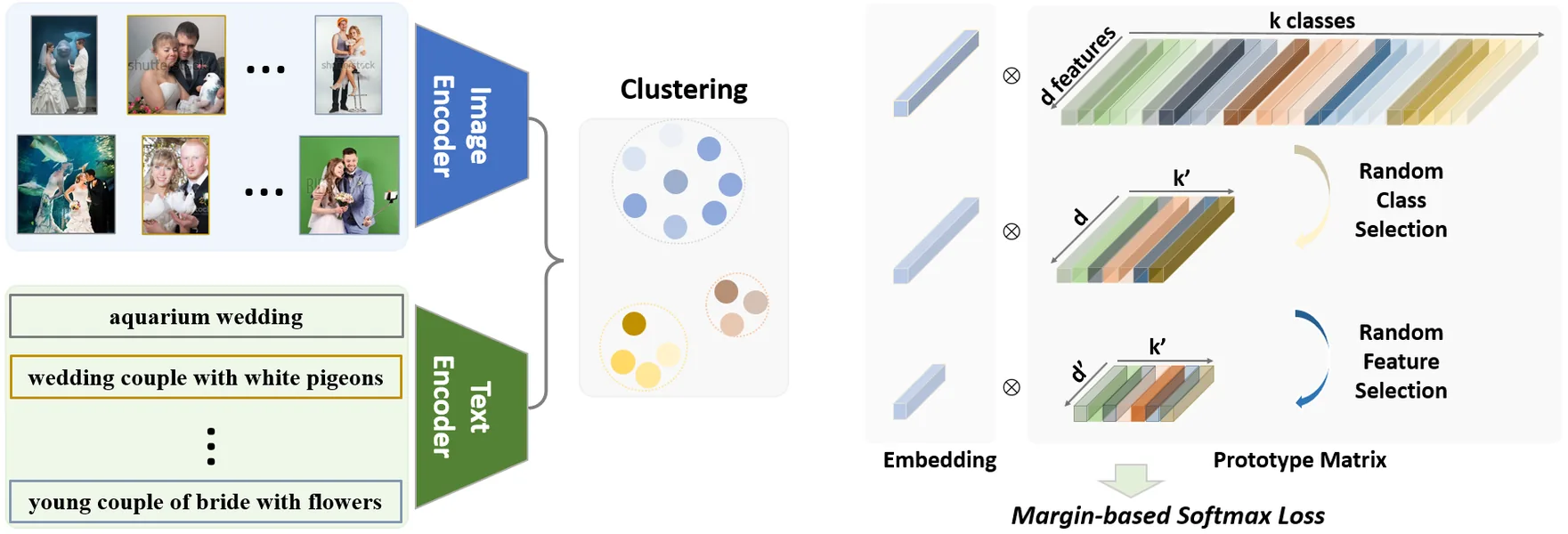
UNICOM averages the CLIP image and text features of each LAION-400M sample and runs k-means once. With feature quantization the whole dataset clusters in about ten minutes, into one million classes of roughly 400 images each. Classes found this way conflict: a pair of birds lands in a wedding-couple class, and close-ups of wedding flowers also turn up in a wedding-venue class, because one image carries several labels and the granularity of a class is arbitrary.
UNICOM 对每个 LAION-400M 样本取 CLIP 图像特征与文本特征的平均,只做一次 k-means。借助特征量化,整个数据集约十分钟即可聚完,得到一百万个类,每类约 400 张图。这样聚出的类别彼此冲突:一对鸟被分进“新人合影”类,婚礼鲜花的特写也出现在“婚礼场地”类中,原因是一张图常带有多个标签,类别的粒度也没有统一标准。
Two random selections let the classifier train on such labels (Figure 2). At each step the margin-based softmax (ArcFace, margin 0.3, scale 64) sees the positive class and a random 10% of the other class prototypes, so a conflicting class is ten times less likely to push the image away. A second selection keeps a random subset of the feature dimensions, the same subset for the whole mini-batch and for both the embeddings and the prototypes. Unlike Dropout, this trains each sub-space of the embedding on its own, which keeps short descriptors useful for retrieval: on CUB, after one extra epoch at r₂ = 0.5, UNICOM beats the unsupervised retrieval method STML at every length from 256 down to 32 dimensions, although STML trains on CUB and UNICOM does not.
两次随机选择让分类器能在这样的标签上训练(图 2)。每一步,带间隔的 softmax(ArcFace,间隔 0.3,尺度 64)只看到正类和随机 10% 的其他类原型,冲突类把图像推开的概率因此降为十分之一。第二次选择随机保留一部分特征维度,整个 mini-batch 共用同一组维度,嵌入和原型同时截取。与 Dropout 不同,这样嵌入的每个子空间都单独得到训练,短描述子依然适合检索:在 CUB 上,用 r₂ = 0.5 多训练一个 epoch 后,UNICOM 在 256 到 32 维的每个长度上都超过无监督检索方法 STML,尽管 STML 在 CUB 上训练过,UNICOM 没有。
Ablations: clustering features, class count and random selection (Tables 1, 2)消融:聚类特征、类别数与随机选择(表 1、表 2)
Joint image–text features cluster better than either alone, and one million classes beat 100K and 10M. Sampling 10% of the negative classes adds 7.8 points of linear-probe accuracy over using all of them (85.7 vs 77.9). A feature ratio r₂ = 0.5 adds 0.4 to 256-d retrieval (61.8 vs 61.4), while Dropout lowers it.
图文联合特征的聚类效果好于单用图像或文本,一百万类好于十万类和一千万类。只采样 10% 的负类,比使用全部负类的线性探测高 7.8 分(85.7 对 77.9)。特征比例 r₂ = 0.5 让 256 维检索提高 0.4(61.8 对 61.4),Dropout 则让它下降。
Table 1Which features to cluster, and how many classes (ViT-B/32 on LAION-400M). Each cell averages the 13 linear-probe datasets of Table 6 or the 7 retrieval benchmarks of Table 5; blue marks the best in each row.表 1用什么特征聚类、聚成多少类(ViT-B/32,LAION-400M)。每格是表 6 中 13 个线性探测数据集或表 5 中 7 个检索基准的平均;蓝色为每行最佳。
| Task任务 | Clustered with CLIP用 CLIP 聚类 | Clustered with OpenCLIP用 OpenCLIP 聚类 | Classes (CLIP, joint)类别数(CLIP 图文) | ||||||
|---|---|---|---|---|---|---|---|---|---|
| Image图像 | Text文本 | Joint图文 | Image图像 | Text文本 | Joint图文 | 100K | 1M | 10M | |
| Linear probe线性探测 | 84.4 | 85.3 | 85.7 | 83.9 | 84.0 | 84.1 | 75.9 | 85.7 | 83.6 |
| Unsupervised retrieval无监督检索 | 61.8 | 62.3 | 62.8 | 58.9 | 60.1 | 61.1 | 53.2 | 62.8 | 60.7 |
Table 2Random class and feature selection against Dropout (ViT-B/32, averages as in Table 1). r₁ = 0.1 and r₂ = 1.0 are the same model; the last row retrieves with 256-d instead of the full 512-d descriptors. Blue marks the best in each row.表 2随机类别选择、随机特征选择与 Dropout 的对比(ViT-B/32,平均方式同表 1)。r₁ = 0.1 与 r₂ = 1.0 是同一个模型;最后一行用 256 维而不是完整的 512 维描述子检索。蓝色为每行最佳。
| Task任务 | Class ratio r₁类别比例 r₁ | Feature ratio r₂特征比例 r₂ | Dropout r₃Dropout r₃ | ||||||
|---|---|---|---|---|---|---|---|---|---|
| 0.05 | 0.1 | 0.3 | 1.0 | 1.0 | 0.5 | 0.25 | 0.25 | 0.5 | |
| Linear probe线性探测 | 85.1 | 85.7 | 84.9 | 77.9 | 85.7 | 85.5 | 84.2 | 85.4 | 85.1 |
| Unsupervised retrieval无监督检索 | 62.3 | 62.8 | 62.1 | 55.9 | 62.8 | 62.7 | 62.0 | 62.5 | 62.3 |
| Unsupervised retrieval, 256-d无监督检索,256 维 | – | – | – | – | 61.4 | 61.8 | 61.0 | 60.7 | 60.1 |
MLCD: several classes per imageMLCD:每张图多个类别
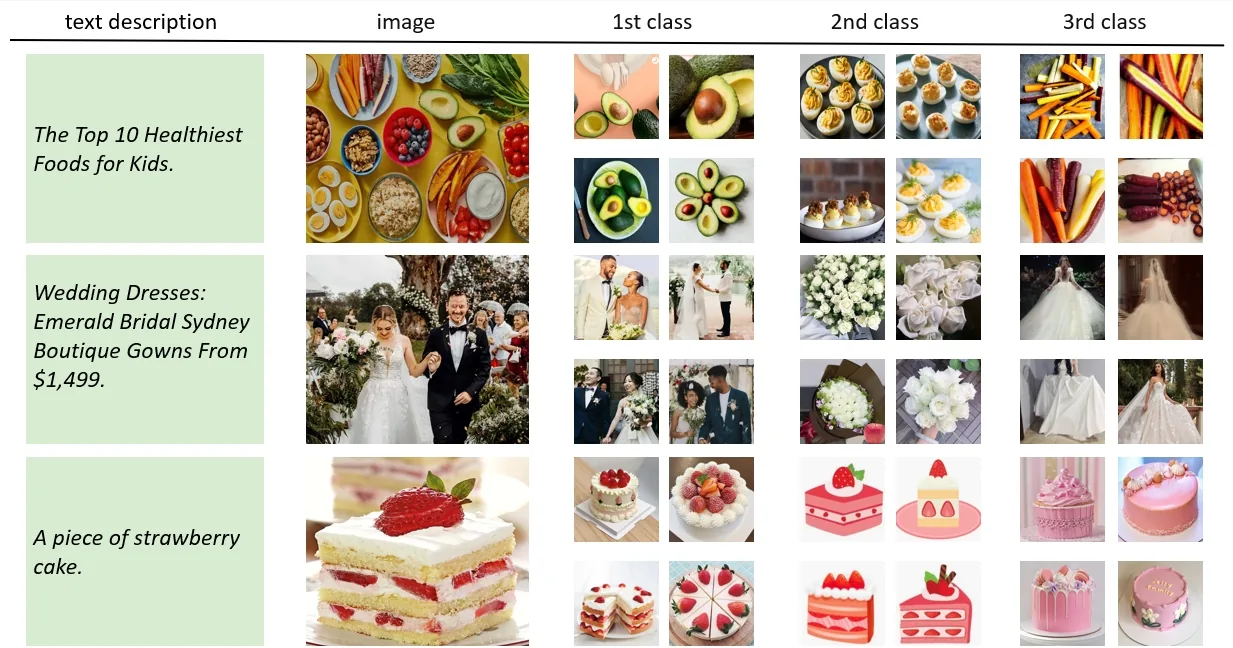
One pseudo-label rarely covers a web image. The wedding photo in Figure 3 shows a couple, white roses and a gown, while its caption names only the gowns. MLCD keeps UNICOM’s clustering, one million classes from CLIP ViT-L/14 features of LAION-400M, but ranks all class centres by similarity to each image and keeps the eight closest as positives. Every other class is a negative, and a random 10% of them enter each step.
一个伪标签很难概括一张网络图片。图 3 中的婚礼照片里有一对新人、白玫瑰和婚纱,而它的文本只提到婚纱。MLCD 沿用 UNICOM 的聚类,即用 CLIP ViT-L/14 特征把 LAION-400M 聚成一百万类,但会把所有类中心按与图像的相似度排序,取最近的 8 个作为正类。其余类都是负类,每一步随机取其中 10% 参与计算。
The loss follows Circle loss. A plain multi-label loss (MLC) only shrinks every gap sⱼ − sᵢ between a negative and a positive similarity, which leaves the decision boundary ambiguous: the pairs {sⱼ, sᵢ} = {0.1, 0.4} and {0.5, 0.8} meet the same margin of 0.3, yet the second pair’s negative scores higher than the first pair’s positive. MLCD adds one term that raises every sᵢ and one that lowers every sⱼ, and the loss then splits into a positive part and a negative part. In the paper’s training curves, MLCD’s mean similarity to positive class centres rises well above MLC’s, while its mean similarity to negative centres stays near zero.
损失函数参照 Circle loss。普通的多标签损失(MLC)只缩小每一对负类与正类相似度之差 sⱼ − sᵢ,决策边界因此含糊:{sⱼ, sᵢ} = {0.1, 0.4} 与 {0.5, 0.8} 都满足 0.3 的间隔,但第二组的负类比第一组的正类得分还高。MLCD 再加两项,一项抬高每个 sᵢ,一项压低每个 sⱼ,损失于是分成正类和负类两部分。论文给出的训练曲线显示,MLCD 与正类中心的平均相似度明显高于 MLC,与负类中心的平均相似度则保持在 0 附近。
Ablations: classes, negative sampling, positives per image and the split loss (Tables 3, 4)消融:类别数、负类采样、每张图的正类数与拆分损失(表 3、表 4)
One million classes, a 10% negative sample and eight positives per image work best. More positives add noisy labels: 16 drops to 72.1 and 32 to 68.7. Choosing positives by a similarity threshold, so that each image gets a different number, peaks at 73.3, below the fixed eight (75.2). The split loss improves on MLC in all three ImageNet settings.
一百万类、10% 的负类采样、每张图 8 个正类效果最好。正类再多就会引入噪声标签:16 个降到 72.1,32 个降到 68.7。按相似度阈值选正类(每张图的正类数不同),最好只有 73.3,低于固定的 8 个(75.2)。拆分后的损失在 ImageNet 的三种设置下都优于 MLC。
Table 3MLCD ablations: ViT-B/32 trained on LAION-400M for 5 epochs, ImageNet linear-probe top-1 %. The last block picks positives by a similarity threshold instead of a fixed count. Blue marks the paper’s best setting.表 3MLCD 消融:ViT-B/32 在 LAION-400M 上训练 5 个 epoch,ImageNet 线性探测 top-1 %。最后一组按相似度阈值而不是固定数量选正类。蓝色为论文中的最佳设置。
| Classes类别数 | 100K | 200K | 500K | 1M | 2M | 5M |
|---|---|---|---|---|---|---|
| ImageNet linear probeImageNet 线性探测 | 66.9 | 71.1 | 74.4 | 75.2 | 74.9 | 74.7 |
| Negative ratio r负类比例 r | 0.01 | 0.05 | 0.1 | 0.2 | 0.5 | 1.0 |
| ImageNet linear probeImageNet 线性探测 | 73.4 | 75.1 | 75.2 | 74.9 | 68.3 | 63.2 |
| Positives per image每张图的正类数 | 1 | 2 | 4 | 8 | 16 | 32 |
| ImageNet linear probeImageNet 线性探测 | 71.4 | 72.9 | 73.2 | 75.2 | 72.1 | 68.7 |
| Similarity threshold相似度阈值 | 0.95 | 0.93 | 0.91 | 0.89 | 0.87 | 0.85 |
| ImageNet linear probeImageNet 线性探测 | 72.2 | 72.7 | 73.3 | 72.4 | 68.7 | 63.2 |
Table 4The plain multi-label loss (MLC) against MLCD’s split loss on ImageNet: ViT-B/32 trained on LAION-400M for 32 epochs, both with 10% negative sampling.表 4普通多标签损失(MLC)与 MLCD 拆分损失在 ImageNet 上的对比:ViT-B/32 在 LAION-400M 上训练 32 个 epoch,两者都采样 10% 的负类。
| Loss损失 | Fine-tune微调 | Linear probe线性探测 | Zero-shot零样本 |
|---|---|---|---|
| MLC | 80.9 | 76.9 | 63.9 |
| MLCD | 81.2 | 78.1 | 64.5 |
Results结果
UNICOM: retrieval and linear probingUNICOM:检索与线性探测
UNICOM’s encoders are trained from scratch for 32 epochs on the clustered LAION-400M. Its ViT-L/14 averages 69.9 on seven unsupervised retrieval benchmarks, 7.5 points above OpenCLIP’s ViT-L/14 and 5.4 above OpenCLIP’s larger ViT-H/14 (Table 5). In linear probing on 13 datasets it is ahead of OpenCLIP, trained on the same data, by 3.6, 2.7 and 1.4 points on average for ViT-B/32, B/16 and L/14 (Table 6). Fine-tuned for retrieval, its largest model is above the best earlier result on all ten metrics of Table 7, results that come from various backbones. Fine-tuned on ImageNet-1K, its ViT-L/14 reaches 88.3, above ViT-L/16 pre-trained on JFT-300M (87.8) or IG-3.6B (88.1) (Table 8).
UNICOM 的编码器在聚类后的 LAION-400M 上从零训练 32 个 epoch。它的 ViT-L/14 在 7 个无监督检索基准上平均 69.9,比 OpenCLIP 的 ViT-L/14 高 7.5,比更大的 OpenCLIP ViT-H/14 还高 5.4(表 5)。在 13 个数据集的线性探测上,它平均领先使用相同数据的 OpenCLIP:ViT-B/32、B/16、L/14 分别高 3.6、2.7、1.4(表 6)。为检索微调后,它最大的模型在表 7 的十项指标上都超过此前最好的结果,这些结果来自各不相同的骨干网络。在 ImageNet-1K 上微调后,它的 ViT-L/14 达到 88.3,超过在 JFT-300M(87.8)或 IG-3.6B(88.1)上预训练的 ViT-L/16(表 8)。
Table 5Unsupervised image retrieval with the frozen pre-trained encoders: Recall@1, mAP@100 on GLDv2. UNICOM rows shaded; blue marks the best score in each column.表 5冻结预训练编码器的无监督图像检索:Recall@1,GLDv2 为 mAP@100。UNICOM 行加底色,蓝色为每列最佳。
| Backbone骨干 | CUB | Cars | SOP | In-Shop | iNaturalist | VehicleID | GLDv2 | Avg.平均 | |||
|---|---|---|---|---|---|---|---|---|---|---|---|
| Small小 | Medium中 | Large大 | Private私有 | Public公开 | |||||||
| CLIP (WIT-400M) | |||||||||||
| ViT-B/32 | 56.7 | 79.0 | 60.5 | 45.4 | 53.0 | 54.8 | 52.2 | 44.6 | 7.5 | 7.5 | 46.1 |
| ViT-B/16 | 66.1 | 85.2 | 63.2 | 56.1 | 63.1 | 55.1 | 50.9 | 43.8 | 8.4 | 10.6 | 50.3 |
| ViT-L/14 | 76.0 | 90.3 | 65.6 | 62.9 | 72.9 | 62.4 | 58.9 | 51.8 | 12.1 | 13.6 | 56.7 |
| ViT-L/14-336 | 77.3 | 90.9 | 67.8 | 66.3 | 76.8 | 64.1 | 60.3 | 53.8 | 17.0 | 15.6 | 59.0 |
| OpenCLIP (LAION-400M) | |||||||||||
| ViT-B/32 | 62.3 | 89.2 | 65.9 | 64.6 | 54.9 | 71.0 | 67.1 | 59.9 | 9.17 | 8.4 | 55.2 |
| ViT-B/16 | 71.4 | 92.9 | 68.7 | 74.2 | 64.1 | 73.3 | 70.1 | 63.7 | 12.1 | 11.0 | 60.2 |
| ViT-L/14 | 79.4 | 94.9 | 70.6 | 77.1 | 71.0 | 72.0 | 69.1 | 62.0 | 14.5 | 13.8 | 62.4 |
| ViT-H/14 | 83.1 | 95.7 | 72.7 | 78.8 | 77.0 | 72.7 | 69.7 | 61.9 | 17.7 | 15.3 | 64.5 |
| UNICOM (LAION-400M) | |||||||||||
| ViT-B/32 | 83.7 | 95.9 | 70.0 | 72.8 | 64.6 | 74.9 | 72.0 | 65.4 | 15.1 | 13.3 | 62.8 |
| ViT-B/16 | 86.5 | 96.8 | 70.4 | 74.6 | 73.6 | 74.5 | 70.6 | 58.7 | 18.7 | 17.2 | 64.2 |
| ViT-L/14 | 88.5 | 96.9 | 72.7 | 83.6 | 77.1 | 83.7 | 80.2 | 74.6 | 21.1 | 20.1 | 69.9 |
| ViT-L/14-336 | 89.2 | 97.3 | 74.5 | 86.7 | 81.0 | 84.1 | 81.4 | 75.6 | 23.2 | 22.0 | 71.5 |
Table 6Linear probe on 13 image classification datasets, top-1 %. -336: one extra epoch at 336 px. UNICOM rows shaded; blue marks the best score in each column.表 613 个图像分类数据集上的线性探测,top-1 %。-336 表示在 336 px 下多训练一个 epoch。UNICOM 行加底色,蓝色为每列最佳。
| Backbone骨干 | CIFAR-10 | CIFAR-100 | Caltech-101 | Cars | Flowers | Food-101 | Birdsnap | SUN397 | DTD | Aircraft | Pets | EuroSAT | ImageNet | Avg.平均 |
|---|---|---|---|---|---|---|---|---|---|---|---|---|---|---|
| CLIP (WIT-400M) | ||||||||||||||
| ViT-B/32 | 95.1 | 80.5 | 93.0 | 81.8 | 96.9 | 88.8 | 58.5 | 76.6 | 76.5 | 52.0 | 90.0 | 97.0 | 76.1 | 81.8 |
| ViT-B/16 | 96.2 | 83.1 | 94.7 | 86.7 | 98.1 | 92.8 | 67.8 | 78.4 | 79.2 | 59.5 | 93.1 | 97.1 | 80.2 | 85.1 |
| ViT-L/14 | 98.0 | 87.5 | 96.5 | 90.9 | 99.2 | 95.2 | 77.0 | 81.8 | 82.1 | 69.4 | 95.1 | 98.2 | 83.9 | 88.8 |
| ViT-L/14-336 | 97.9 | 87.4 | 96.0 | 91.5 | 99.2 | 95.9 | 79.9 | 82.2 | 83.0 | 71.6 | 95.1 | 98.1 | 85.4 | 89.5 |
| CLIP-R: public CLIP re-tested in the UNICOM code baseCLIP-R:公开的 CLIP 模型在 UNICOM 代码中重测 | ||||||||||||||
| ViT-B/32 | 96.0 | 82.5 | 94.1 | 86.0 | 97.8 | 92.7 | 61.1 | 79.1 | 78.4 | 58.9 | 93.0 | 95.3 | 75.3 | 83.9 |
| ViT-B/16 | 96.0 | 82.5 | 94.1 | 86.0 | 97.8 | 92.7 | 69.5 | 79.1 | 78.4 | 58.9 | 93.0 | 95.3 | 79.6 | 84.8 |
| ViT-L/14 | 98.1 | 87.2 | 96.0 | 90.7 | 99.2 | 95.3 | 77.8 | 81.5 | 80.9 | 68.0 | 94.9 | 96.7 | 84.1 | 88.5 |
| ViT-L/14-336 | 97.8 | 87.1 | 96.3 | 91.4 | 99.2 | 95.9 | 80.9 | 82.2 | 82.4 | 71.2 | 95.1 | 96.8 | 84.9 | 89.3 |
| OpenCLIP (LAION-400M) | ||||||||||||||
| ViT-B/32 | 95.3 | 82.2 | 93.3 | 87.5 | 96.5 | 86.2 | 61.4 | 75.3 | 78.8 | 52.4 | 88.0 | 96.5 | 73.8 | 82.1 |
| ViT-B/16 | 96.4 | 84.0 | 94.1 | 91.8 | 98.1 | 90.7 | 71.2 | 78.7 | 81.6 | 59.3 | 90.0 | 96.2 | 78.5 | 85.4 |
| ViT-L/14 | 97.9 | 87.9 | 95.5 | 93.6 | 98.8 | 93.3 | 78.0 | 81.0 | 83.0 | 64.4 | 93.3 | 97.1 | 81.5 | 88.1 |
| UNICOM (LAION-400M) | ||||||||||||||
| ViT-B/32 | 96.8 | 86.6 | 94.6 | 93.3 | 98.5 | 85.8 | 70.2 | 74.6 | 78.0 | 70.7 | 93.1 | 96.8 | 75.0 | 85.7 |
| ViT-B/16 | 97.3 | 87.7 | 95.1 | 94.3 | 98.9 | 91.2 | 79.3 | 77.1 | 81.2 | 73.4 | 93.9 | 97.0 | 79.1 | 88.1 |
| ViT-L/14 | 98.5 | 90.8 | 95.7 | 94.6 | 99.3 | 93.4 | 82.4 | 80.0 | 82.2 | 74.5 | 94.2 | 96.7 | 81.8 | 89.5 |
| ViT-L/14-336 | 98.5 | 90.7 | 95.7 | 95.1 | 99.4 | 94.3 | 85.1 | 79.7 | 82.0 | 78.1 | 94.5 | 97.2 | 82.7 | 90.2 |
Table 7Supervised image retrieval after fine-tuning UNICOM on each benchmark (Recall@1; mAP@100 on GLDv2), against the best earlier result, which uses its own backbone. Blue marks the best score in each row.表 7在各基准上微调 UNICOM 后的有监督图像检索(Recall@1,GLDv2 为 mAP@100),对比此前最好的结果(各自使用不同骨干)。蓝色为每行最佳。
| Benchmark基准 | ViT-B/32 | ViT-B/16 | ViT-L/14 | ViT-L/14-336 | Previous best此前最佳 |
|---|---|---|---|---|---|
| CUB | 85.8 | 88.8 | 89.7 | 90.1 | 85.6ViT-S/16 · Ermolov et al. 2022 |
| Cars | 97.3 | 97.7 | 97.9 | 98.2 | 94.8SE-ResNet-50 · Jun et al. 2019 |
| SOP | 87.1 | 88.8 | 89.9 | 91.2 | 88.0ViT-B/16 · Patel et al. 2022 |
| In-Shop | 94.8 | 95.5 | 96.0 | 96.7 | 92.7ViT-S/16 · Ermolov et al. 2022 |
| iNaturalist | 72.8 | 82.5 | 85.4 | 88.9 | 83.9ViT-B/16 · Patel et al. 2022 |
| VehicleID-Small | 95.4 | 96.4 | 96.5 | 97.0 | 96.2ViT-B/16 · Patel et al. 2022 |
| VehicleID-Medium | 94.1 | 95.1 | 95.7 | 96.1 | 95.2ViT-B/16 · Patel et al. 2022 |
| VehicleID-Large | 93.6 | 95.0 | 95.4 | 96.0 | 94.7ViT-B/16 · Patel et al. 2022 |
| GLDv2-Private | 32.6 | 35.7 | 36.1 | 36.4 | 32.5ResNet101 · Lee et al. 2022 |
| GLDv2-Public | 29.7 | 32.4 | 33.0 | 33.1 | 24.6ResNet50 · Tan et al. 2021 |
Table 8Fine-tuned on ImageNet-1K after pre-training on the listed data. UNICOM rows shaded.表 8在所列数据上预训练后,于 ImageNet-1K 微调的结果。UNICOM 行加底色。
| Model模型 | Pre-training data预训练数据 | Pre-train res.预训练分辨率 | Fine-tune res.微调分辨率 | ImageNet-1K top-1ImageNet-1K top-1 | FLOPs (B)FLOPs (B) |
|---|---|---|---|---|---|
| Supervised pre-training有监督预训练 | |||||
| ViT-L/32Dosovitskiy et al. 2021 | ImageNet-21K | 224 | 384 | 81.3 | 54.4 |
| ViT-B/16Dosovitskiy et al. 2021 | ImageNet-21K | 224 | 384 | 84.0 | 55.6 |
| ViT-L/16Dosovitskiy et al. 2021 | ImageNet-21K | 224 | 384 | 85.2 | 191.5 |
| ViT-L/16Dosovitskiy et al. 2021 | JFT-300M | 224 | 512 | 87.8 | 362.9 |
| ViT-L/16Zhai et al. 2022 | JFT-3B | 224 | 384 | 88.5 | 191.5 |
| Weakly supervised pre-training弱监督预训练 | |||||
| ViT-B/16Singh et al. 2022 | IG-3.6B | 224 | 384 | 85.3 | 55.6 |
| ViT-L/16Singh et al. 2022 | IG-3.6B | 224 | 512 | 88.1 | 362.9 |
| OpenCLIP ViT-B/32 | LAION-400M | 224 | 384 | 83.0 | 15.5 |
| OpenCLIP ViT-B/16 | LAION-400M | 224 | 384 | 85.4 | 55.6 |
| OpenCLIP ViT-L/14 | LAION-400M | 224 | 518 | 87.7 | 507.8 |
| UNICOM ViT-B/32 | LAION-400M | 224 | 384 | 83.6 | 15.5 |
| UNICOM ViT-B/16 | LAION-400M | 224 | 384 | 85.9 | 55.6 |
| UNICOM ViT-L/14 | LAION-400M | 224 | 518 | 88.3 | 507.8 |
MLCD: against CLIP, OpenCLIP, FLIP and UNICOMMLCD:对比 CLIP、OpenCLIP、FLIP 与 UNICOM
MLCD’s ViT-L/14 is trained for 32 epochs on LAION-400M; for zero-shot tasks a text encoder is then trained against the frozen image encoder (LiT). Over 26 linear-probe datasets it averages 84.6, against 82.3 for OpenCLIP and 83.3 for UNICOM on the same data and 83.5 for CLIP reproduced on WIT-400M; it is ahead of OpenCLIP on 25 datasets and of UNICOM on 23 (Figure 4). Over 25 zero-shot datasets it averages 67.5, against 66.0 for FLIP and 63.6 for OpenCLIP; it is ahead of OpenCLIP on 23 and of FLIP on 15 (Table 9). In zero-shot retrieval it ties FLIP on Flickr30k text R@1 and is best on every other metric except Flickr30k text R@5 and R@10 (Table 10). On ImageNet it reaches 87.1 fine-tuned, 84.6 linear and 75.6 zero-shot, and it is the most robust LAION-400M model on four of the five shifted test sets; FLIP stays ahead on ImageNet-R (Table 11).
MLCD 的 ViT-L/14 在 LAION-400M 上训练 32 个 epoch;零样本任务所需的文本编码器随后在冻结的图像编码器上训练(LiT)。在 26 个线性探测数据集上,它平均 84.6,相同数据下 OpenCLIP 为 82.3、UNICOM 为 83.3,在 WIT-400M 上复现的 CLIP 为 83.5;它在 25 个数据集上领先 OpenCLIP,在 23 个上领先 UNICOM(图 4)。在 25 个零样本数据集上,它平均 67.5,FLIP 为 66.0,OpenCLIP 为 63.6;其中 23 个领先 OpenCLIP,15 个领先 FLIP(表 9)。零样本检索中,它在 Flickr30k 文本检索 R@1 上与 FLIP 持平,除 Flickr30k 文本检索的 R@5、R@10 外其余指标都最好(表 10)。在 ImageNet 上,它的微调、线性探测和零样本结果分别为 87.1、84.6、75.6,五个分布偏移测试集中有四个是 LAION-400M 模型里最鲁棒的,ImageNet-R 上 FLIP 仍领先(表 11)。
Table 9ViT-L/14 on 26 linear-probe and 25 zero-shot datasets (FER2013 has no zero-shot score). CLIP is trained on WIT-400M, all others on LAION-400M. †: from the CLIP paper; ‡: reproduced by the MLCD authors; §: from the FLIP paper. Blue marks the best LAION-400M model in each group, as in the paper.表 9ViT-L/14 在 26 个线性探测数据集和 25 个零样本数据集上的结果(FER2013 没有零样本分数)。CLIP 在 WIT-400M 上训练,其余都在 LAION-400M 上训练。†:取自 CLIP 论文;‡:MLCD 作者复现;§:取自 FLIP 论文。蓝色为每组中最好的 LAION-400M 模型,与论文标注一致。
| Dataset数据集 | Linear probe线性探测 | Zero-shot零样本 | ||||||||
|---|---|---|---|---|---|---|---|---|---|---|
| CLIP† | CLIP‡ | OpenCLIP‡ | UNICOM | MLCD | CLIP† | CLIP§ | OpenCLIP§ | FLIP§ | MLCD | |
| Food-101 | 95.2 | 95.3 | 93.3 | 93.4 | 94.3 | 92.9 | 91.0 | 87.4 | 89.3 | 90.3 |
| CIFAR-10 | 98.0 | 98.1 | 97.9 | 98.5 | 98.9 | 96.2 | 95.2 | 94.1 | 97.2 | 95.3 |
| CIFAR-100 | 87.5 | 87.2 | 87.9 | 90.8 | 92.0 | 77.9 | 75.6 | 77.1 | 84.1 | 83.7 |
| Birdsnap | 77.0 | 77.8 | 78.0 | 82.4 | 83.4 | 48.3 | 51.2 | 61.3 | 63.0 | 62.9 |
| SUN397 | 81.8 | 81.5 | 81.0 | 80.0 | 82.1 | 67.7 | 66.6 | 70.7 | 73.1 | 72.1 |
| Cars | 90.9 | 90.7 | 93.6 | 94.6 | 94.8 | 77.3 | 75.0 | 86.2 | 90.7 | 90.1 |
| Aircraft | 69.4 | 68.0 | 64.4 | 74.5 | 79.6 | 36.1 | 32.3 | 21.8 | 29.1 | 39.4 |
| VOC2007 | 89.6 | 89.7 | 91.7 | 91.4 | 92.5 | 84.1 | 83.3 | 83.5 | 83.1 | 84.5 |
| DTD | 82.1 | 80.9 | 83.0 | 82.2 | 84.6 | 55.3 | 55.0 | 54.9 | 60.4 | 62.3 |
| Pets | 95.1 | 94.9 | 93.3 | 94.2 | 95.3 | 93.5 | 93.6 | 90.8 | 92.6 | 93.7 |
| Caltech-101 | 96.5 | 96.0 | 95.5 | 95.7 | 97.2 | 92.6 | 92.4 | 94.0 | 93.8 | 93.9 |
| Flowers | 99.2 | 99.2 | 98.8 | 99.3 | 99.3 | 78.7 | 77.7 | 72.1 | 75.0 | 79.4 |
| MNIST | 99.2 | 99.2 | 99.2 | 99.2 | 99.3 | 87.2 | 76.0 | 71.5 | 80.3 | 78.5 |
| FER2013 | 72.2 | 72.3 | 66.5 | 68.7 | 72.4 | – | – | – | – | – |
| STL-10 | 99.8 | 99.8 | 99.2 | 98.5 | 99.3 | 99.3 | 99.3 | 98.2 | 98.5 | 99.1 |
| EuroSAT | 98.2 | 96.7 | 97.1 | 96.7 | 99.1 | 59.9 | 62.0 | 53.3 | 53.5 | 59.7 |
| RESISC45 | 94.1 | 94.5 | 92.4 | 92.6 | 94.7 | 71.6 | 71.6 | 67.7 | 70.8 | 69.9 |
| GTSRB | 92.5 | 92.9 | 92.5 | 92.7 | 92.5 | 50.3 | 51.6 | 47.3 | 41.4 | 50.7 |
| KITTI | 64.7 | 65.9 | 77.5 | 77.8 | 78.2 | 23.1 | 26.9 | 29.3 | 34.8 | 28.7 |
| Country211 | 42.9 | 41.9 | 32.5 | 33.4 | 34.5 | 32.7 | 30.9 | 21.6 | 23.1 | 27.9 |
| PCAM | 85.8 | 85.3 | 84.3 | 85.4 | 86.0 | 58.8 | 51.6 | 51.1 | 50.3 | 53.7 |
| UCF101 | 91.5 | 91.0 | 88.1 | 87.4 | 90.0 | 76.2 | 76.1 | 71.3 | 74.1 | 75.7 |
| Kinetics-700 | 72.0 | 70.6 | 64.0 | 66.7 | 68.5 | 60.3 | 59.5 | 50.5 | 55.8 | 57.7 |
| CLEVR | 57.8 | 59.6 | 59.8 | 60.3 | 60.1 | 24.3 | 22.2 | 22.0 | 22.7 | 22.2 |
| Hateful Memes | 76.2 | 61.8 | 57.6 | 57.4 | 57.9 | 63.3 | 55.3 | 55.3 | 54.0 | 58.4 |
| SST-2 | 80.8 | 79.8 | 71.9 | 72.4 | 73.4 | 64.0 | 67.3 | 57.1 | 58.5 | 57.9 |
| Average平均 | 84.2 | 83.5 | 82.3 | 83.3 | 84.6 | 66.9 | 65.6 | 63.6 | 66.0 | 67.5 |
Table 10Zero-shot image–text retrieval on the Flickr30k and MSCOCO test splits, ViT-L/14. §: from the FLIP paper. Blue marks the best LAION-400M model in each column, as in the paper.表 10Flickr30k 与 MSCOCO 测试集上的零样本图文检索,ViT-L/14。§:取自 FLIP 论文。蓝色为每列中最好的 LAION-400M 模型,与论文标注一致。
| Model模型 | Data数据 | Text retrieval文本检索 | Image retrieval图像检索 | ||||||||||
|---|---|---|---|---|---|---|---|---|---|---|---|---|---|
| Flickr30k | MSCOCO | Flickr30k | MSCOCO | ||||||||||
| R@1 | R@5 | R@10 | R@1 | R@5 | R@10 | R@1 | R@5 | R@10 | R@1 | R@5 | R@10 | ||
| CLIP§ | WIT-400M | 87.8 | 99.1 | 99.8 | 56.2 | 79.8 | 86.4 | 69.3 | 90.2 | 94.0 | 35.8 | 60.7 | 70.7 |
| OpenCLIP§ | LAION-400M | 87.3 | 97.9 | 99.1 | 58.0 | 80.6 | 88.1 | 72.0 | 90.8 | 95.0 | 41.3 | 66.6 | 76.1 |
| FLIP§ | LAION-400M | 89.1 | 98.5 | 99.6 | 60.2 | 82.6 | 89.9 | 75.4 | 92.5 | 95.9 | 44.2 | 69.2 | 78.4 |
| MLCD | LAION-400M | 89.1 | 98.4 | 99.5 | 60.8 | 83.2 | 91.3 | 75.9 | 93.1 | 96.8 | 44.5 | 69.6 | 79.9 |
Table 11ImageNet under fine-tuning, linear probe and zero-shot, and zero-shot robustness on five shifted test sets, ViT-L/14. §: from the FLIP paper. Blue marks the best LAION-400M model in each column, as in the paper.表 11ImageNet 上的微调、线性探测和零样本结果,以及五个分布偏移测试集上的零样本鲁棒性,ViT-L/14。§:取自 FLIP 论文。蓝色为每列中最好的 LAION-400M 模型,与论文标注一致。
| Model模型 | Data数据 | ImageNet | Zero-shot robustness零样本鲁棒性 | ||||||
|---|---|---|---|---|---|---|---|---|---|
| Fine-tune微调 | Linear probe线性探测 | Zero-shot零样本 | IN-V2 | IN-A | IN-R | ObjectNet | IN-Sketch | ||
| CLIP§ | WIT-400M | – | 83.9 | 75.3 | 69.5 | 71.9 | 86.8 | 68.6 | 58.5 |
| OpenCLIP§ | LAION-400M | 86.2 | 82.1 | 72.8 | 64.0 | 48.3 | 84.3 | 58.8 | 56.9 |
| FLIP§ | LAION-400M | – | – | 74.6 | 66.8 | 51.2 | 86.5 | 59.1 | 59.9 |
| MLCD | LAION-400M | 87.1 | 84.6 | 75.6 | 68.9 | 56.4 | 85.1 | 62.7 | 60.4 |
Single- against multi-label on LAION-400M and COYO-700M, ViT-B/32 (Table 12)单标签与多标签在 LAION-400M 和 COYO-700M 上的对比,ViT-B/32(表 12)
With ViT-B/32, MLCD beats UNICOM by 2.2 points on LAION-400M (81.4 vs 79.2) and by 1.6 on COYO-700M (82.9 vs 81.3), averaged over 26 linear-probe datasets. COYO-700M helps action recognition: with MLCD, Kinetics-700 rises from 60.9 to 64.2.
使用 ViT-B/32 时,在 26 个线性探测数据集上平均,MLCD 在 LAION-400M 上比 UNICOM 高 2.2(81.4 对 79.2),在 COYO-700M 上高 1.6(82.9 对 81.3)。COYO-700M 有助于动作识别:使用 MLCD 时,Kinetics-700 从 60.9 升到 64.2。
Table 12Single-label (UNICOM) against multi-label (MLCD) cluster discrimination on two pre-training sets, ViT-B/32, linear probe on 26 datasets. Blue marks the better of the two on each dataset, as in the paper.表 12单标签(UNICOM)与多标签(MLCD)聚类判别在两个预训练数据集上的对比,ViT-B/32,26 个数据集的线性探测。蓝色为每个数据集上两者中较好的一个,与论文标注一致。
| Dataset数据集 | LAION-400M | COYO-700M | ||
|---|---|---|---|---|
| UNICOM | MLCD | UNICOM | MLCD | |
| Food-101 | 85.8 | 87.8 | 88.1 | 90.2 |
| CIFAR-10 | 96.8 | 97.5 | 95.4 | 96.9 |
| CIFAR-100 | 86.6 | 88.2 | 85.8 | 86.8 |
| Birdsnap | 70.2 | 72.4 | 71.4 | 72.1 |
| SUN397 | 74.6 | 77.6 | 76.6 | 77.4 |
| Cars | 93.3 | 93.8 | 93.1 | 93.5 |
| Aircraft | 70.7 | 71.4 | 72.7 | 74.7 |
| VOC2007 | 88.3 | 91.9 | 88.1 | 90.4 |
| DTD | 78.0 | 80.4 | 81.7 | 83.5 |
| Pets | 93.1 | 93.2 | 93.3 | 93.6 |
| Caltech-101 | 94.6 | 96.9 | 95.6 | 97.7 |
| Flowers | 98.5 | 98.8 | 97.5 | 98.8 |
| MNIST | 98.7 | 99.3 | 99.3 | 99.3 |
| FER2013 | 64.3 | 66.4 | 70.3 | 70.9 |
| STL-10 | 97.8 | 98.6 | 98.7 | 99.1 |
| EuroSAT | 96.8 | 98.6 | 97.8 | 99.0 |
| RESISC45 | 90.6 | 92.1 | 91.5 | 92.7 |
| GTSRB | 90.0 | 90.5 | 89.9 | 90.1 |
| KITTI | 76.4 | 77.7 | 76.7 | 77.5 |
| Country211 | 22.5 | 30.9 | 30.4 | 33.7 |
| PCAM | 82.9 | 83.4 | 82.1 | 84.4 |
| UCF101 | 84.2 | 86.3 | 86.3 | 87.5 |
| Kinetics-700 | 57.2 | 60.9 | 61.8 | 64.2 |
| CLEVR | 52.6 | 54.1 | 57.4 | 59.2 |
| Hateful Memes | 52.4 | 57.9 | 64.3 | 68.4 |
| SST-2 | 62.1 | 70.4 | 69.1 | 73.4 |
| Average平均 | 79.2 | 81.4 | 81.3 | 82.9 |
As the vision tower of LLaVA-1.5, an MLCD ViT-L/14 pre-trained on LAION-400M and COYO-700M, then trained one more epoch at 336 px, replaces CLIP ViT-L/14 under the LLaVA-1.5 recipe. With Qwen2-7B it is better on 12 of the 18 scores, with one tie; with Qwen2-72B it is better on 15 (Table 13). It loses on the OCR-heavy TextVQA and AI2D with both language models, which the paper plans to address by adding OCR models to the clustering.
作为 LLaVA-1.5 的视觉编码器,在 LAION-400M 与 COYO-700M 上预训练、再在 336 px 下训练一个 epoch 的 MLCD ViT-L/14,按 LLaVA-1.5 的流程替换 CLIP ViT-L/14。搭配 Qwen2-7B 时,它在 18 项分数中有 12 项更好、1 项持平;搭配 Qwen2-72B 时有 15 项更好(表 13)。两种语言模型下,它在偏重 OCR 的 TextVQA 和 AI2D 上都落后,论文计划在聚类时加入 OCR 模型来弥补。
Table 13CLIP ViT-L/14 against MLCD ViT-L/14 (pre-trained on LAION-400M and COYO-700M) as the vision tower of LLaVA-1.5, with the LLaVA-1.5 settings and two Qwen2 language models. TVQA is TextVQA. Blue marks the better tower for each language model, as in the paper.表 13以 CLIP ViT-L/14 和 MLCD ViT-L/14(在 LAION-400M 与 COYO-700M 上预训练)作为 LLaVA-1.5 的视觉编码器,沿用 LLaVA-1.5 的设置,搭配两个 Qwen2 语言模型。TVQA 即 TextVQA。蓝色为每个语言模型下较好的视觉编码器,与论文标注一致。
| Benchmark基准 | Qwen2-7B | Qwen2-72B | ||
|---|---|---|---|---|
| CLIP | MLCD | CLIP | MLCD | |
| VQAv2val | 77.99 | 78.32 | 79.47 | 79.51 |
| GQAeval | 62.66 | 63.56 | 63.81 | 66.80 |
| VizWizval | 48.58 | 46.27 | 67.14 | 67.37 |
| SQAimg | 72.24 | 74.22 | 76.10 | 74.69 |
| TVQAval | 48.98 | 42.52 | 62.31 | 57.32 |
| L-Wildtest | 58.70 | 58.90 | 65.41 | 66.00 |
| AI2Dtest | 64.86 | 62.82 | 72.41 | 71.41 |
| MathVmini | 33.60 | 33.60 | 38.30 | 46.5 |
| HBIall | 39.96 | 39.46 | 45.10 | 45.21 |
| MMMUval | 40.70 | 42.30 | 39.70 | 44.70 |
| cMMMUval | 33.70 | 33.10 | 37.45 | 41.20 |
| MMBenchEN | 72.03 | 73.88 | 76.63 | 78.59 |
| MMBenchCN | 70.29 | 71.47 | 75.39 | 77.24 |
| SEED-Benchall | 64.25 | 65.79 | 66.54 | 68.67 |
| SEED-Benchimg | 69.40 | 71.05 | 72.28 | 76.53 |
| SEED-Benchvid | 44.72 | 45.89 | 44.71 | 45.91 |
| MMEperception | 1512 | 1558 | 1596 | 1633 |
| MMEcognition | 335 | 384 | 378 | 383 |
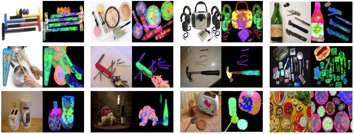
The patch features carry semantics without dense supervision. After one epoch at 448 px, thresholding the first PCA component of the 32×32 patch tokens separates objects from the background, and mapping three components to RGB colours objects of the same category alike (Figure 5).
它的 patch 特征不需要稠密监督就带有语义。在 448 px 下训练一个 epoch 后,对 32×32 个 patch token 的第一主成分取阈值即可把物体与背景分开,再把三个主成分映射为 RGB,同类物体呈现相近的颜色(图 5)。
After the papers论文之后
The repository kept scaling MLCD as a vision tower for multimodal LLMs. ViT-bigG/14 models at 336 and 448 px add 2D RoPE; inside LLaVA-NeXT with Qwen2.5-7B, the 448-px model scores 73.80 on ChartQA, 83.34 on DocVQA and 582 on OCRBench, above CLIP ViT-L/14 and SigLIP SO400M (Table 14). In April 2025 MLCD ViT-bigG was merged into Hugging Face Transformers as MLCDVisionModel.
代码仓库继续把 MLCD 扩展为多模态大模型的视觉编码器。336 px 和 448 px 的 ViT-bigG/14 模型加入了 2D RoPE;在搭配 Qwen2.5-7B 的 LLaVA-NeXT 中,448 px 模型在 ChartQA、DocVQA、OCRBench 上分别得到 73.80、83.34、582,高于 CLIP ViT-L/14 和 SigLIP SO400M(表 14)。2025 年 4 月,MLCD ViT-bigG 以 MLCDVisionModel 的形式并入 Hugging Face Transformers。
Table 14From the repository README, not from either paper: vision towers inside LLaVA-NeXT, trained on its official data with Qwen2.5-7B. MLCD rows shaded; blue marks the best score in each column.表 14取自代码仓库 README,不在两篇论文中:在 LLaVA-NeXT 中替换视觉编码器,使用官方训练数据和 Qwen2.5-7B。MLCD 行加底色,蓝色为每列最佳。
| Vision tower视觉编码器 | 2D RoPE2D RoPE | ChartQA | DocVQA | InfoVQA | OCRBench | MMMU |
|---|---|---|---|---|---|---|
| CLIP (ViT-L-14-336px) | – | 66.52 | 75.21 | 38.88 | 525.00 | 44.20 |
| SigLIP (ViT-SO400M-384px) | – | 69.28 | 76.71 | 41.38 | 554.00 | 46.78 |
| DFN5B (ViT-H-14-378px) | – | 64.36 | 70.87 | 38.59 | 473.00 | 48.00 |
| MLCD (ViT-L-14-336px) | – | 67.84 | 76.46 | 43.48 | 531.00 | 44.30 |
| MLCD (ViT-bigG-14-336px) | ✓ | 71.07 | 79.63 | 44.38 | 572.00 | 46.78 |
| MLCD (ViT-bigG-14-448px) | ✓ | 73.80 | 83.34 | 46.59 | 582.00 | 46.00 |
The objective also outlived the two papers. Extended from whole images to regions it became RICE (ICCV 2025 highlight), the vision encoder of LLaVA-OneVision-1.5. OneVision-Encoder is trained by cluster discrimination over more than one million concepts, and Mage-ViT uses negative-sampling cluster discrimination with the same 10% ratio.
这个训练目标也延续到了两篇论文之后。从整张图扩展到区域后,它成为 RICE(ICCV 2025 Highlight),也就是 LLaVA-OneVision-1.5 的视觉编码器。OneVision-Encoder 在一百多万个概念上做聚类判别训练,Mage-ViT 也采用带负采样的聚类判别,负采样比例同样是 10%。
Open-source resources开源资源
Code and models are public. The repository is MIT-licensed; on Hugging Face the MLCD ViT-B/32 and ViT-L/14 weights are Apache-2.0 and the ViT-bigG/14 weights MIT.
代码与模型全部公开。代码仓库采用 MIT 许可;Hugging Face 上 MLCD 的 ViT-B/32 与 ViT-L/14 权重采用 Apache-2.0,ViT-bigG/14 权重采用 MIT。
MLCD vision encodersMLCD 视觉编码器
Code, models built on MLCD, papers代码、基于 MLCD 的模型与论文
Citation引用
@inproceedings{anxiang_2024_mlcd,
  title     = {Multi-label Cluster Discrimination for Visual Representation Learning},
  author    = {An, Xiang and Yang, Kaicheng and Dai, Xiangzi and Feng, Ziyong and Deng, Jiankang},
  booktitle = {ECCV},
  year      = {2024}
}
@inproceedings{anxiang_2023_unicom,
  title     = {Unicom: Universal and Compact Representation Learning for Image Retrieval},
  author    = {An, Xiang and Deng, Jiankang and Yang, Kaicheng and Li, Jiawei and Feng, Ziyong and
               Guo, Jia and Yang, Jing and Liu, Tongliang},
  booktitle = {ICLR},
  year      = {2023}
}
Authors作者
UNICOM · Xiang An, Jiankang Deng†, Kaicheng Yang, Jiawei Li, Ziyong Feng, Jia Guo, Jing Yang, Tongliang Liu
MLCD · Xiang An, Kaicheng Yang, Xiangzi Dai, Ziyong Feng, Jiankang Deng†
† Corresponding author. UNICOM: DeepGlint, Huawei, InsightFace, University of Cambridge, University of Sydney. MLCD: DeepGlint, Huawei Noah’s Ark Lab.† 通讯作者。UNICOM:格灵深瞳、华为、InsightFace、剑桥大学、悉尼大学。MLCD:格灵深瞳、华为诺亚方舟实验室。